4.3 Classification of Linear Systems — Part 2

Section 4.3: Classification of Linear Systems (Part 2)

Classification of Linear Systems

OK, we’ve been looking at systems of the form:

$$ \dot{x}=A x $$

Where

$$ x=\left(\begin{matrix} x \\ y \end{matrix}\right) , A=\left(\begin{matrix} a & b \\ c & d \end{matrix}\right) $$

and we’ve said that the important point is the type of eigenvalues that we have for the matrix $A$. So far we have looked at the cases where we have a positive and a negative eigenvalue, and found that the flows in the plane sometimes flow towards the fixed point at $\left(x,y\right)=\left(0,0\right)$ and sometimes flow away from it. If both eigenvalues are negative, then we will always flow towards the fixed point, and if both are positive then we will always flow away from the fixed point.

Here we want to focus on the case where the eigenvalues may be complex. One thing to note here is that because the eigenvalues come from a real quadratic equation, the solutions will come in complex conjugate pairs. This means that if one is complex, of the form $\alpha{}+i \omega{}$ where $\alpha{} \text{ and } \omega{}$ are both real, the other eigenvalue will be of the form $\alpha{}-i \omega{}, \text{ with }$

$$ \alpha{}=\frac{\tau{}}{2} \text{ and } \omega{}=\frac{1}{2}\sqrt{4\Delta{}-{\tau{}}^{2}} $$

where remember τ is the trace of your matrix, and Δ is the determinant.

So you will never have a situation with one real and one complex eigenvalue. So the classification here will come down to whether ω is positive, negative or zero. For now we will look at the case where $\omega{}\neq{}0$. We can rewrite the system using the fact that:

$$ e^{\left(\alpha{}+i \omega{}\right)t}=e^{\alpha{} t}e^{i \omega{} t}=e^{\alpha{} t}\left(\text{ cos } \omega{} t+i \text{ sin } \omega{} t\right) $$

and thus:

$$ x=c_{1}e^{\alpha{} t}\left(\text{ cos } \omega{} t+i \text{ sin } \omega{} t\right)v_{1}+c_{2}e^{\alpha{} t}\left(\text{ cos } \omega{} t-i \text{ sin } \omega{} t\right) v_{2}= e^{\alpha{} t}\left(c_{1}\left(\text{ cos } \omega{} t\right) v_{1}+c_{2}\left(\text{ cos } \omega{} t\right) v_{2}+i\left(c_{1}\left(\text{ sin } \omega{} t\right) v_{1}-c_{2}\left(\text{ sin } \omega{} t\right) v_{2}\right)\right) $$

Although it looks like our solution has an imaginary part, in fact when we choose an initial condition, we will find that this is not the case. Let ’s look at an example. Let’s try and solve for the system:

$$ \dot{x}=\left(\begin{matrix} 1 & 2 \\ -2 & 1 \end{matrix}\right) x $$

Now τ=2 and Δ=1+4=5, so α=1 and $\omega{}=\frac{1}{2}\sqrt{4 5-4}=2. $The eigenvalues and eigenvectors of this system are thus:

$$ {\lambda{}}_{1}=1+2i, v_{1}=\left(\begin{matrix} -i \\ 1 \end{matrix}\right) , {\lambda{}}_{2}=1-2i, v_{2}=\left(\begin{matrix} i \\ 1 \end{matrix}\right) $$

So the solution of the DE is:

$$ x =c_{1}e^{t}\left(\text{ cos } 2 t+i \text{ sin } 2t\right)\left(\begin{matrix} -i \\ 1 \end{matrix}\right) +c_{2}e^{t}\left(\text{ cos } 2 t-i \text{ sin } 2t\right)\left(\begin{matrix} i \\ 1 \end{matrix}\right) $$

This all seems pretty confusing, as we want our solutions to be purely real. Let’s say our initial conditions are $x=\left(\begin{matrix} 1 \\ 1 \end{matrix}\right) $, which is equivalent to $x=1, y=1$. Let’s solve for $c_{1}, c_{2}$ by setting t=0

$$ \left(\begin{matrix} 1 \\ 1 \end{matrix}\right)=c_{1}\left(1\right)\left(\begin{matrix} -i \\ 1 \end{matrix}\right) +c_{2}\left(1\right)\left(\begin{matrix} i \\ 1 \end{matrix}\right) $$

This gives two equations:

$$ 1=-i c1+i c2, 1=c1+c2 $$

which solves to give:

$$ c_{1}=\frac{1}{2}+\frac{\mathrm{i}}{2},c_{2}=\frac{1}{2}-\frac{\mathrm{i}}{2} $$

Plugging this back in gives us:

$$ x =\left(\frac{1}{2}+\frac{\mathrm{i}}{2}\right)e^{t}\left(\text{ cos } 2 t+i \text{ sin } 2t\right)\left(\begin{matrix} -i \\ 1 \end{matrix}\right) +\left(\frac{1}{2}-\frac{\mathrm{i}}{2}\right)e^{t}\left(\text{ cos } 2 t-i \text{ sin } 2t\right)\left(\begin{matrix} i \\ 1 \end{matrix}\right) $$

which looks even worse than before, but if you work out each component of the vector you get:

$$ \\=\frac{e^{t}}{2}\left(\begin{matrix} \left(-i+1\right)\left(\text{ cos } 2 t+i \text{ sin } 2t\right)+\left(i+1\right)\left(\text{ cos } 2 t-i \text{ sin } 2t\right) \\ \left(1+i\right)\left(\text{ cos } 2 t+i \text{ sin } 2t\right)+\left(1-i\right)\left(\text{ cos } 2 t-i \text{ sin } 2t\right) \end{matrix}\right) \\=\frac{e^{t}}{2}\left(\begin{matrix} -i \text{ cos } 2t +\text{ sin } 2t+\text{ cos } 2t +i \text{ sin } 2t+i \text{ cos } 2t+ \text{ sin } 2t+\text{ cos } 2t-i \text{ sin } 2t \\ \text{ cos } 2t+i \text{ sin } 2t+i \text{ cos } 2t-\text{ sin } 2t+\text{ cos } 2t-i \text{ sin } 2t-i \text{ cos } 2t-\text{ sin } 2t \end{matrix}\right) \\=e^{t}\left(\begin{matrix} \text{ sin } 2t+\text{ cos } 2t \\ \text{ cos } 2t-\text{ sin } 2t \end{matrix}\right) $$

and Hallelujah, it’s completely real! That was messy, but you should go through it at least once in your life so you can tell your friends and family.

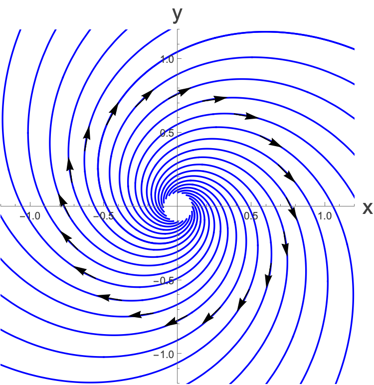
What on earth does this mean? Well, remember the top component of the vector is the position in $x$ and the bottom component is the position in y. We can ask what this looks like as a path in the $\left(x,y\right)$ plane and the answer is:

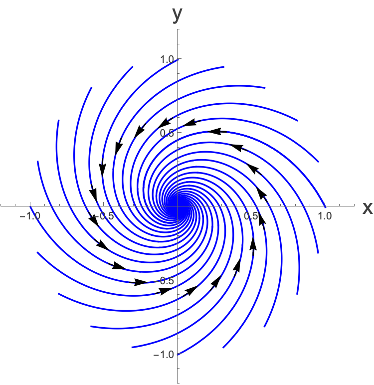
Should we be surprised by this? Well, the fact that we had a positive real part to our eigenvalues tell us that we are going to have an exponentially growing solution, and the fact that there was an imaginary part tells us that we will be rotating.

The phase portrait for such a system is known as a spiral:

There are three possible forms of rotation: If α is positive, then we will be spiralling out from the centre. If α is negative we will be spiralling into the centre, and if $\alpha{}=0$ we will have a periodic solution. These would look like, for $\alpha{}<0$ :

With phase portrait:

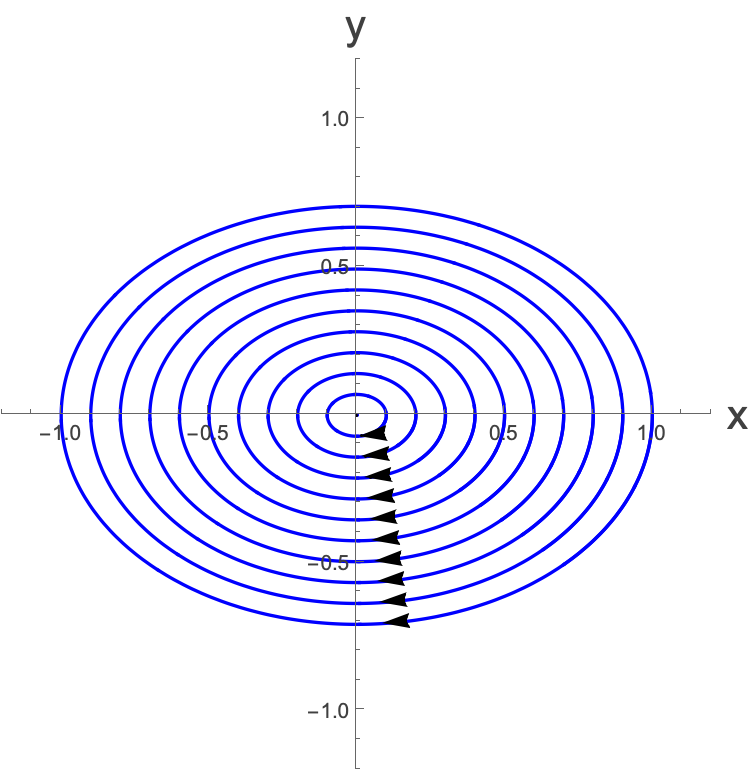
and of course for $\alpha{}=0$:

Note that all of these correspond to initial conditions of $\left(x_{o},y_{o}\right)=\left(1,1\right)$. For the periodic solution, the period $T=\frac{2\pi{}}{\omega{}}$. A phase portrait for such a system is known as a centre. Here is an example where it’s periodic but the amplitude in x and y is different:

OK, so we’ve looked at complex solutions, and basically have completely classified them. You either have spiralling in, spiralling out or periodic solutions.

For real solutions we have also looked at whether you have both eigenvalues positive, or both negative or one of each.

There is a third possibility, which itself has two subclasses. You can have both eigenvalues being the same. There are two ways that this can happen. Clearly this can never happen if you have complex eigenvalues as these come in complex conjugate pairs and will always be different. So, we are talking here about a single real eigenvalue. This will happen when ${\tau{}}^{2}=4\Delta{}$ and so the discriminant vanishes. We can write this in terms of the matrix A as:

$$ A=\left(\begin{matrix} a & b \\ c & d \end{matrix}\right) \text{ with } {\left(a+d\right)}^{2}=4\left(a d-b c\right) $$

One way that this can happen if $b=c=0$ and $a=d$. Then you can write the matrix A directly in terms of the eigenvalues:

$$ A=\left(\begin{matrix} \lambda{} & 0 \\ 0 & \lambda{} \end{matrix}\right) $$

What are the eigenvectors of this matrix? Well, this matrix is just the identity matrix up to a scaling. All vectors are eigenvectors of this matrix with eigenvalue λ. So if you start with position $x_{o}=\left(\begin{matrix} x_{o} \\ y_{o} \end{matrix}\right) $the solution is:

$$ x=\left(\begin{matrix} x_{o} \\ y_{o} \end{matrix}\right) e^{\lambda{} t} $$

which just scales everything into or out from the centre depending on whether λ is positive or negative and the phase portrait looks like:

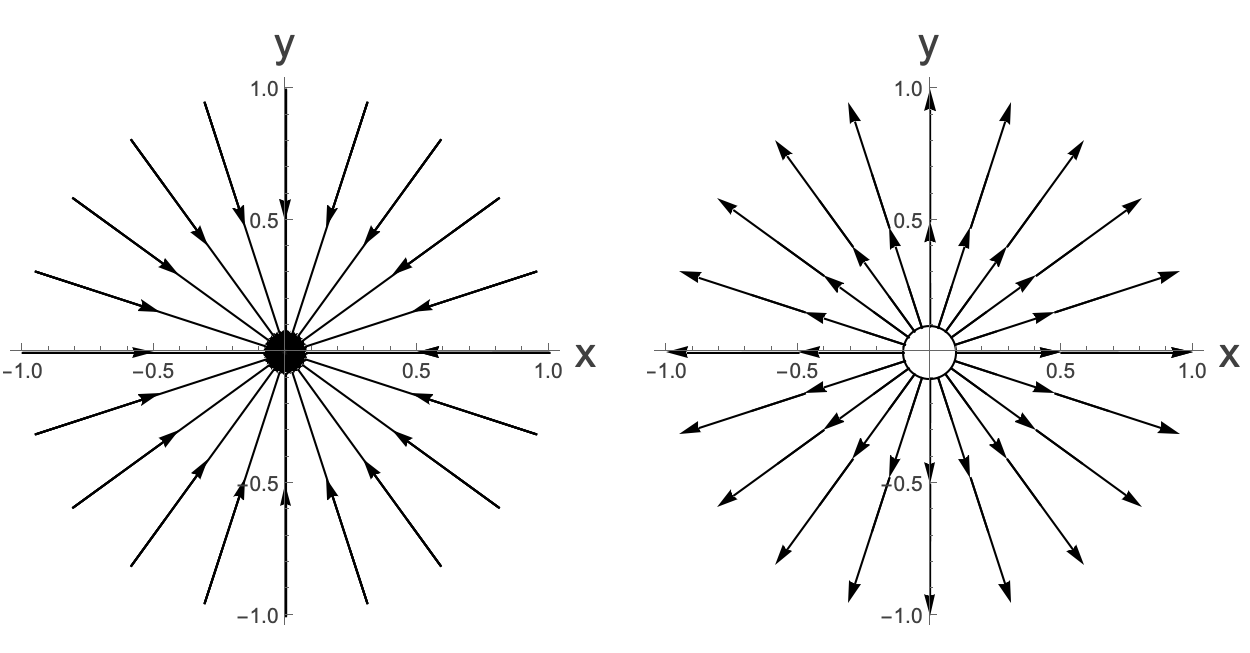
For negative and positive λ respectively. These are known as stars.

The other possibility for a single eigenvalue is when we have $A=\left(\begin{matrix} \lambda{} & b \\ 0 & \lambda{} \end{matrix}\right) $ for non-zero $b$. In this case, it’s not that all vectors are eigenvectors, but now there is only a single eigenvector. This means that there is only one line of arrows which go into the centre rather than the two which we saw previously. As a reminder, when we have two real eigenvalues the phase portraits look like, for instance:

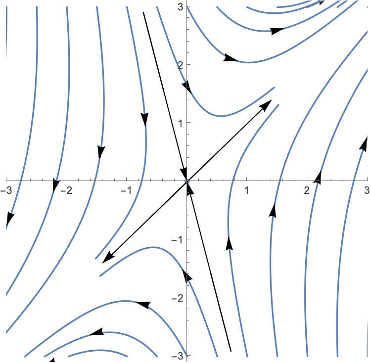
Now, we just have a single line of arrows. Let’s look at an example of this.

Let $A=\left(\begin{matrix} -1 & 1 \\ 0 & -1 \end{matrix}\right) $ I will leave it as a challenge exercise for you to show that the solution is:

$$ x=c_{1}\left(\begin{matrix} 1 \\ 0 \end{matrix}\right) e^{ -t}+c_{2}\left(\left(\begin{matrix} 0 \\ 1 \end{matrix}\right) + \left(\begin{matrix} 1 \\ 0 \end{matrix}\right) t \right)e^{ -t} $$

This gives the following phase portrait:

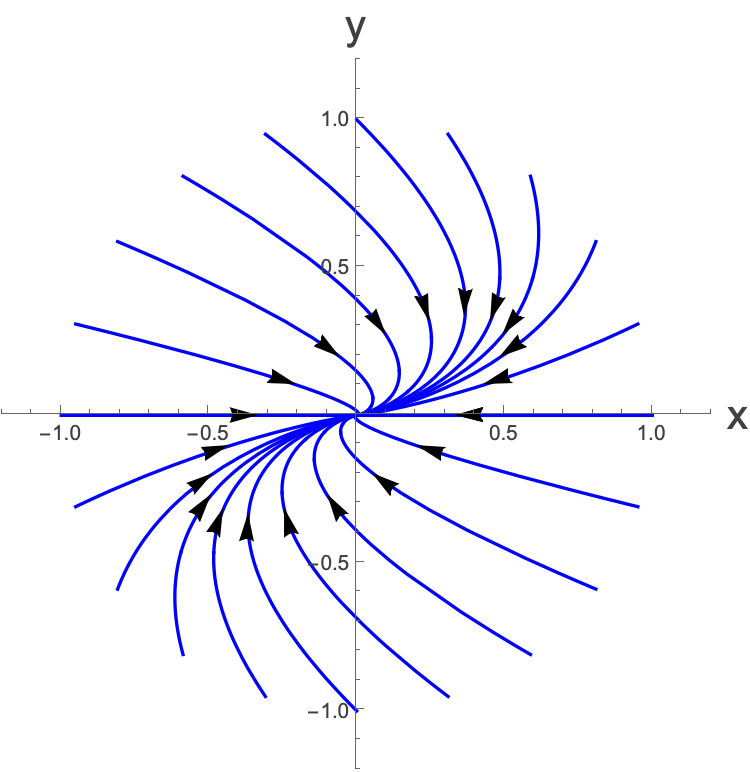
where you can see that there is a single line which is simply scaled which here is the line given by the vector $\left(\begin{matrix} 1 \\ 0 \end{matrix}\right)$. This type of fixed point is known as a degenerate node. The reason for this is that you can think of this as a the limit of the case of two eigenvectors, but where you rotate one of them to be the same as (degenerate with) the other.

Let’s summarise a bit here - What are the options for the eigenvalues:

• Two eigenvalues, both real: Two vectors along which the flow doesn’t change direction. If both correspond to negative eigenvalues then the origin is stable, else it’s unstable.

• Two eigenvalues, both complex: They will be complex conjugate pairs and this will lead to rotating solutions in the $\left(x,y\right)$ plane. If there is a real part then it will either decay in (negative real part) or explode out (positive real part). The frequency and direction of the rotation is dictated by the imaginary part.

• Only a single eigenvalue: Either corresponding to an all vectors being eigenvectors in which case all solutions come in along lines directly to or away from the origin, or there is a single eigenvector and all other lines find themselves getting closer and closer to this line (see the figure above).

• There is one other option which is that the matrix A is zero, in which case all points are fixed points.

• OK, and one other where we have a line of fixed points. This is the case where Δ=0 but τ≠0, for instance $A=\left(\begin{matrix} 1 & 1 \\ 1 & 1 \end{matrix}\right) $. In which case we get a single differential equation:

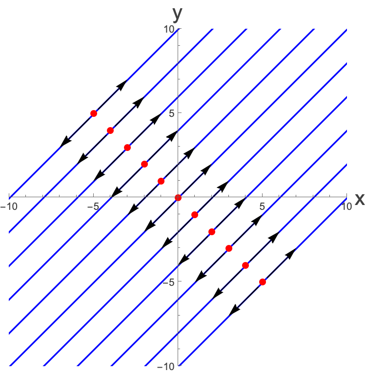
Where the red dots are fixed points, and in fact there’s a continuous line of them $\text{ at } x=-y.$

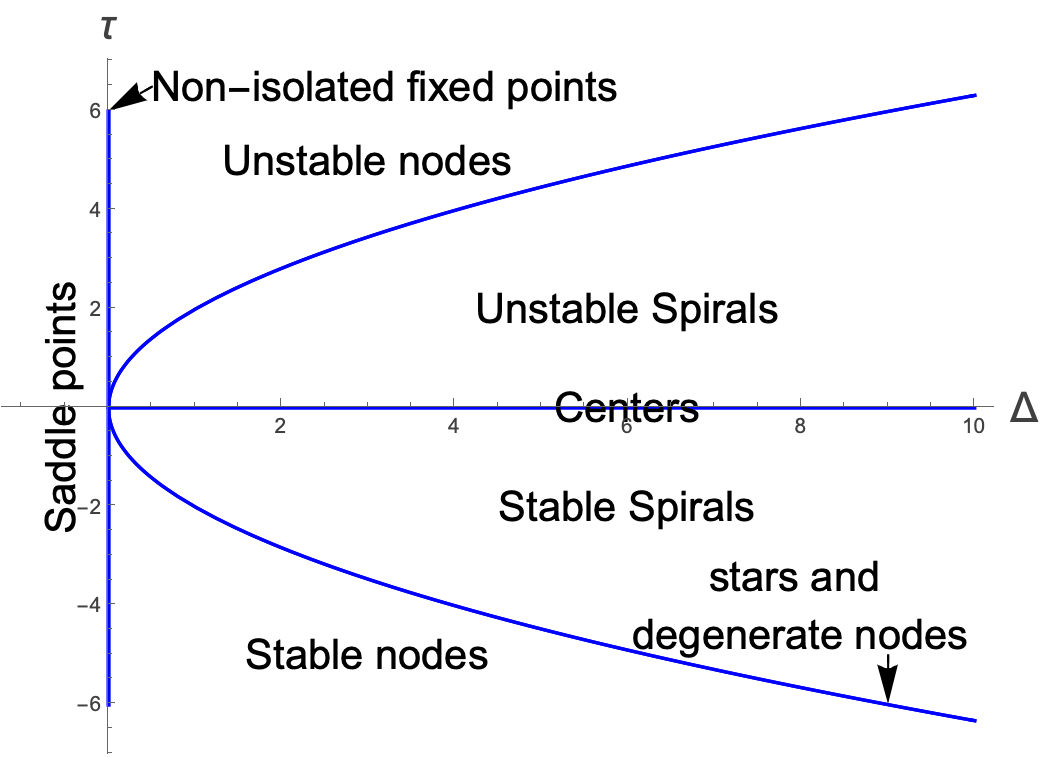
One can plot the regions in the space of Δ’s and τ’s which type of solutions you will get and this looks like: