3.8 Exercise 1d
Exercise 1d
$For: \dot{x}=r+\frac{x}{2}-\frac{x}{1+x}$
- i) Sketch the different vector field types that appear when you vary $r$. We’re actually going to do this first the hard way, then the easier way.
Looking at the phase portrait for different values of $r$ we get the following. The red dashed line corresponds to the discontinuity at $x=-1.$ Red points are fixed points. Arrows indicate flows on the line.
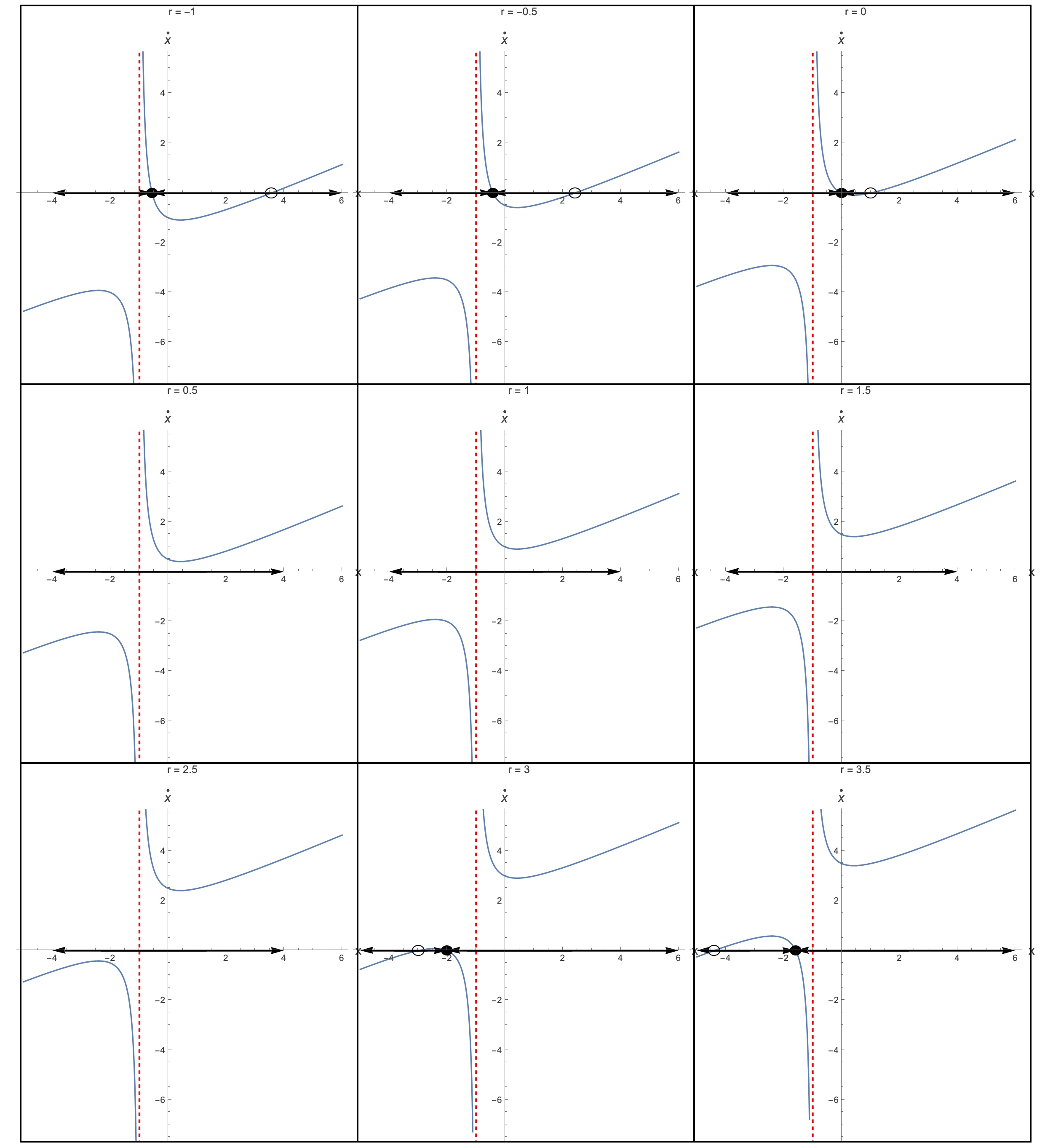
Note that there is a discontinuity at $x=-1, $so there are arrows facing in opposite directions without having a fixed point in between.
Now taking the arrows and fixed points alone and plotting them as a vector field:
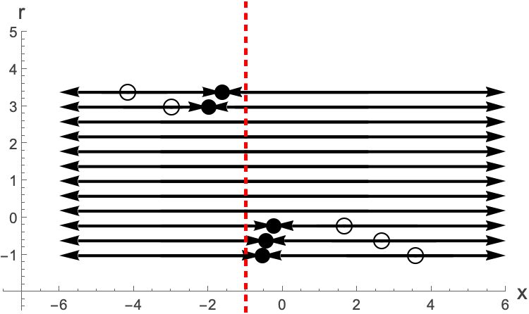
$\dot{x}=r+\frac{x}{2}-\frac{x}{1+x}$
$There \text{ is actually } a \text{ much easier } \text{ way to } \text{ think about } \text{ plotting the } \text{ bifurcation diagram } \text{ than this } \text{ though }. Remember \text{ the equation } \text{ is }: \dot{x}=r+\frac{x}{2}-\frac{x}{1+x}$
The fixed points are found by solving for $\dot{x}=0$. There are two solutions as it results in a quadratic equation.
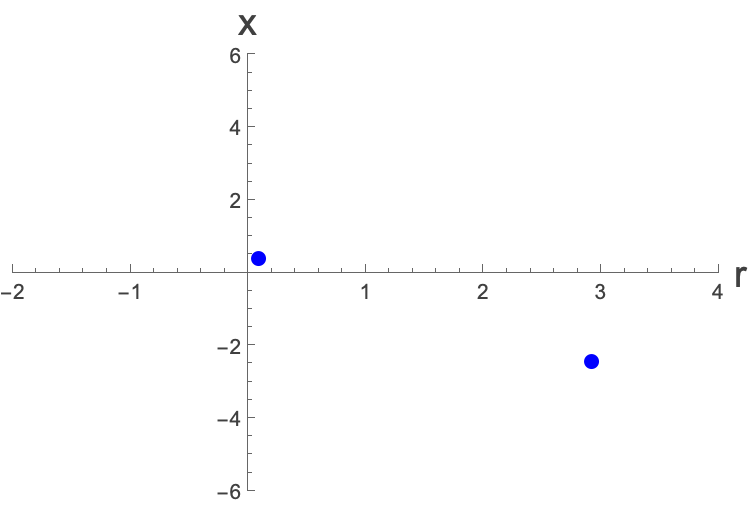
The critical values occur when we have only one solution and not two, which will happen when the term inside the square root is zero:
Which happens when the x-values are:
So the (r,x) coordinates of the critical points are:
Now let’s look at where the fixed points go to when r→∞?
Look at the $\frac{1}{2} \left(1-2 r+\sqrt{1-12 r+4 r^{2}}\right)$ solution
So this fixed point x→ -1 as r→∞.
Now Look at the $\frac{1}{2} \left(1-2 r-\sqrt{1-12 r+4 r^{2}}\right)$ solution
So this fixed point x→ 2-2r as r→∞.
Try and do the same thing for r→-∞. You should find exactly the same answers but reversed (ie. the first one will be the 2-2r and the second one will be the -1.)
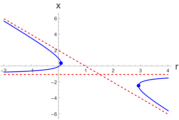
Now put in the critical points, and the asymptotic behaviours of the fixed points as red lines for r→±∞.
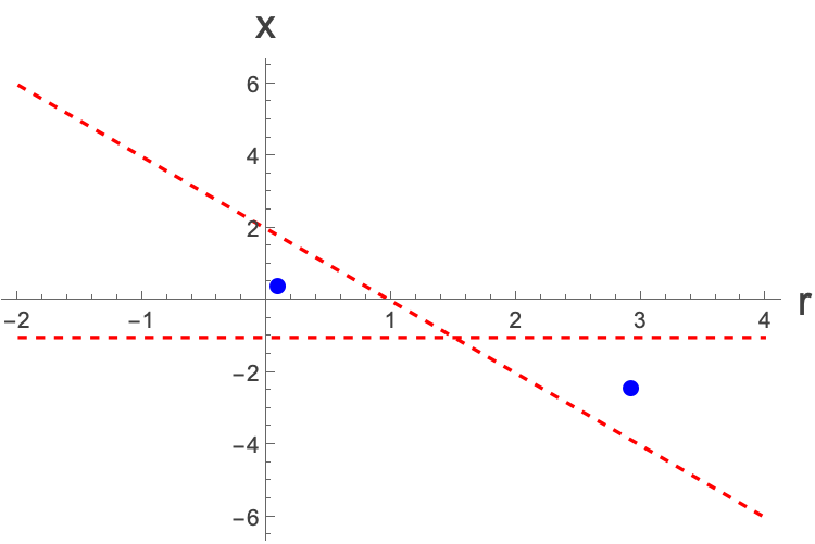
And now put it all together:
We still don’t know which ones of the lines are stable and which are unstable. Let’s take a particular value of r. Let ’s take r=-1 and ask, for the two values of x, which one is stable and which is unstable. The two values of x are:
Plotting these on the bifurcation diagram, we are looking at:

Let’s look at the differential equation now with r=-1 and let x=$\frac{1}{2} \left(3-\sqrt{17}\right)$+η. That is, just a little above the lower fixed point (the smaller value of x), and expand for small positive η:
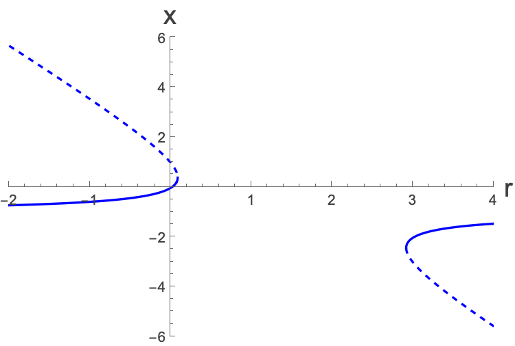
We see that the gradient is negative just above the fixed point. Repeating just below, you will see that it’s positive. This tells us that this fixed point is stable. You can do the same thing for the other branches, and you will get:
We can also expand around the critical points. First take the critical point at $x_{c}=-1+\sqrt{2}$. Expanding the right hand side of the differential equation about this point gives. We can do this by writing $x=x_{c}+\eta{}$ and expanding for small η
Now multiply everything by $2\sqrt{2}$:
Now let $\sqrt{2} \left(-3+2 \sqrt{2}+2 r\right)$=R:
And let $t=2\sqrt{2}T: \left(\frac{d\eta{}}{\text{ dt }}=\frac{d\eta{}}{\text{ dT }}\frac{\text{ dT }}{\text{ dt }}=\frac{d\eta{}}{\text{ dT }}\frac{1}{2\sqrt{2}}\right)$
Which is the normal form for a saddle node bifurcation. You can do the same thing for the other critical point and you will find the same thing.