3.8 Exercise 1b
Exercise 1b
$For: \dot{x}=r-\text{ cosh }\left(x\right)$
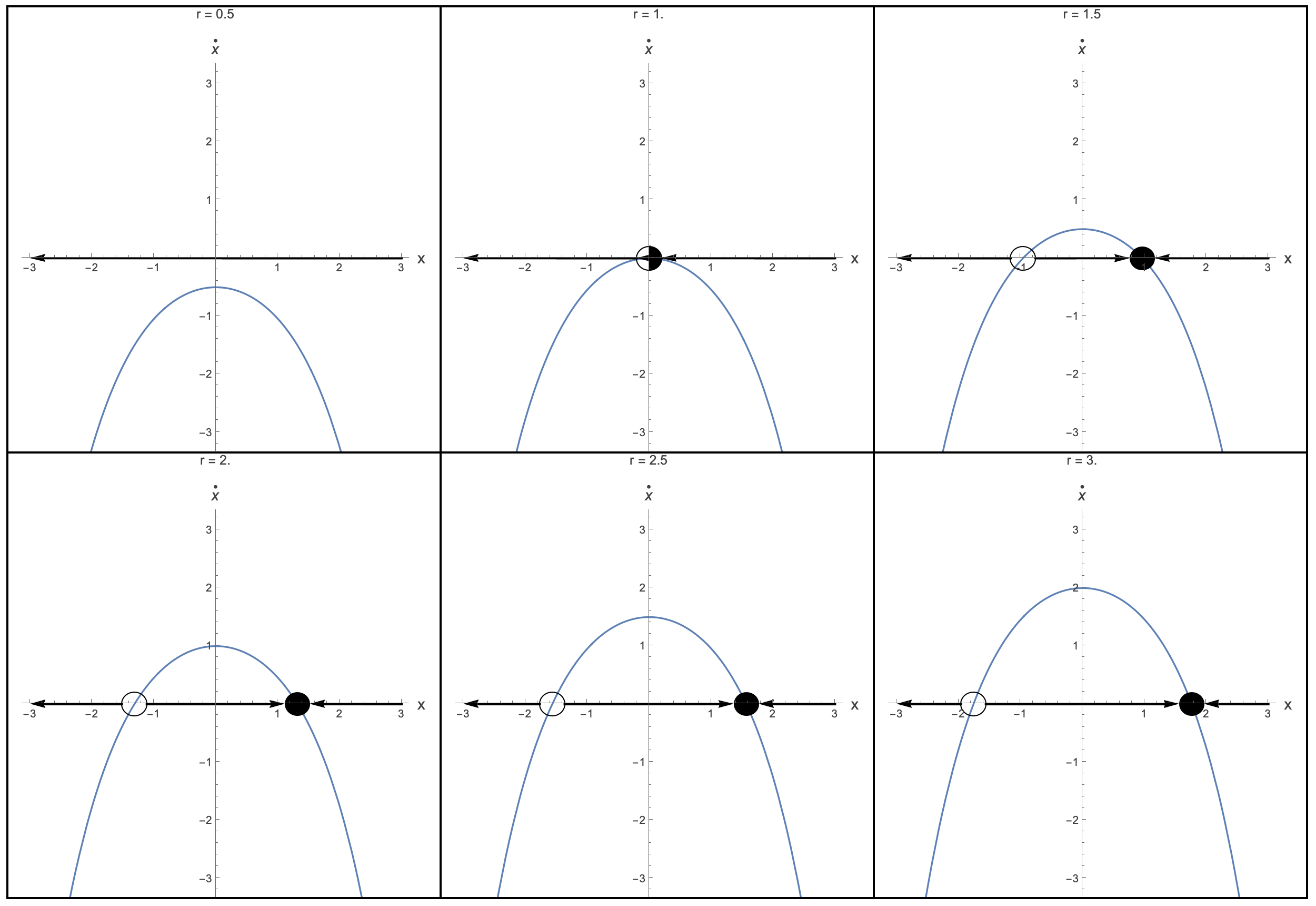
- i) Sketch the different vector field types that appear when you vary $r$. We’re actually going to do this first the hard way, then the easier way.
Looking at the phase portrait for different values of $r$ we get the following.
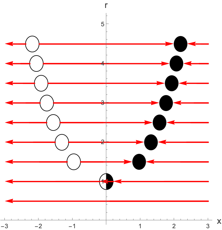
Now taking the arrows and fixed points alone and plotting them as a vector field:
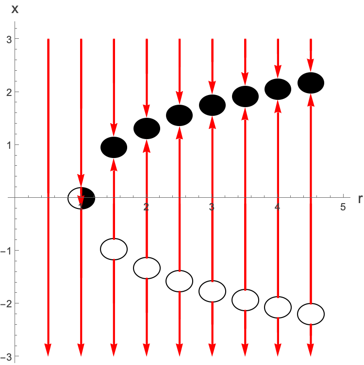
We get the bifurcation diagram by rotating this whole plot above:
We can actually find these fixed points and thus the bifurcation diagram more simply. We need to solve $\dot{x}=r-\text{ cosh }\left(x\right)=0. $So the fixed points occur at:
We can plot these fixed points and this gives us
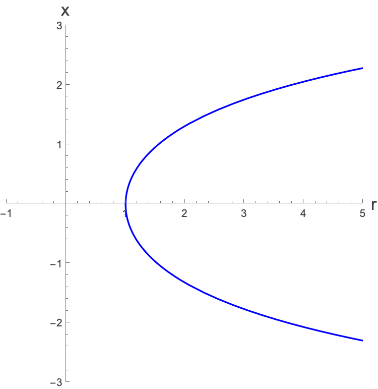
We actually already have whether the fixed points are stable or unstable from the vector field plot above, so let’s put these on:
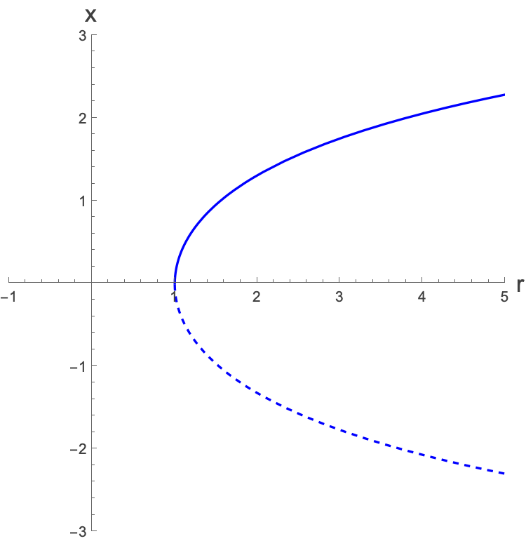
The critical point is when the two solutions are the same (when we go from no fixed points, to one, to two):
Critical point at $r = 1$, and this occurs at: $x=0$:
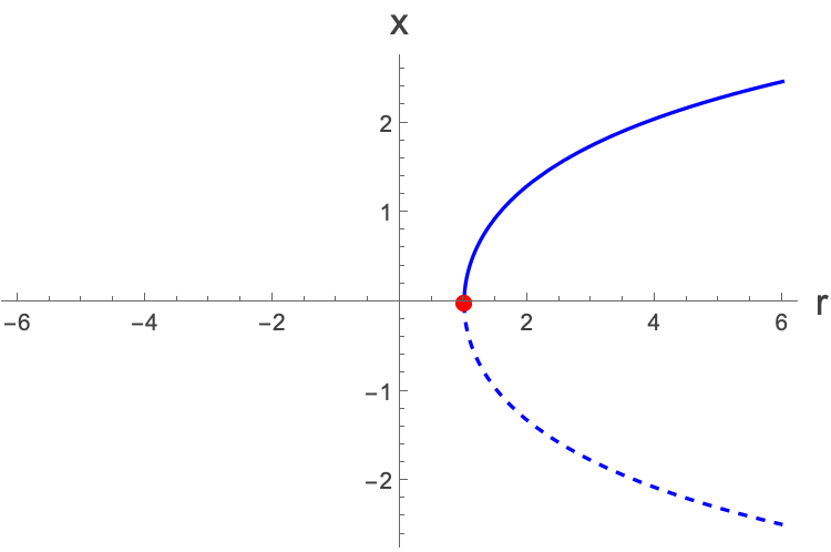
To get the equation about the critical point into normal form we can simply expand the right hand side of the equation about $x=0.$
Defining $R=2\left(r-1$), multiplying everything by 2 and redefining $t=2T$, we get: $\frac{\text{ dx }}{\text{ dT }}=R-x^{2}$. Which is one of the two normal forms for a saddle-node bifurcation.