3.7b Imperfect Bifurcations and Catastrophes (Part 2)

Section 3.7b: Imperfect Bifurcations and Catastrophes

Imperfect Bifurcations and Catastrophes Cont.

OK, where were we? We have been looking at a seemingly very simple differential equation which has two parameters, $h$ and $r$

$$ \dot{x}= h+r x-x^{ 3} $$

We know how to find fixed-points of a differential equation, and we have been finding these for different values of $h$ and then plotting the fixed points in $x$ on a graph as a function of $r$. This was what we had the last time:

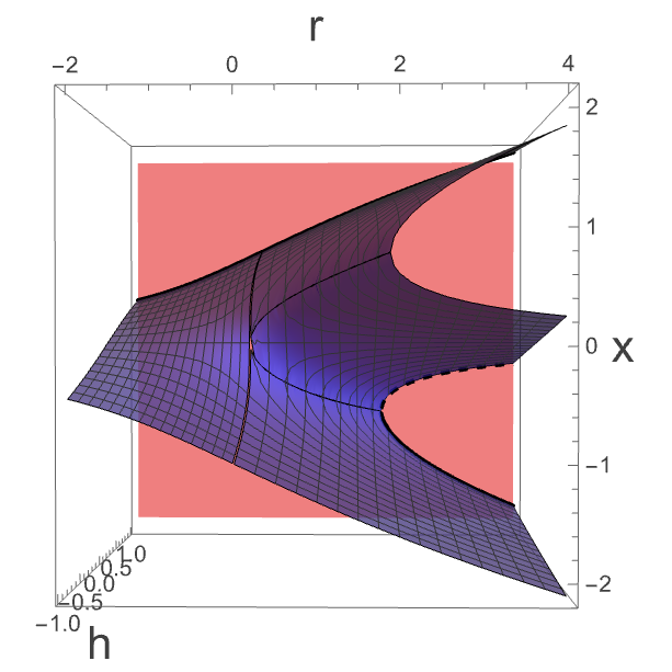
In this case we are changing $h$ and seeing what happens to the fixed points. We can think of this as slicing through a surface where there is a new $h$ dimension. How about plotting this in three dimensions? i.e. as the fixed points of $x$ as a function of $r$ and $h$:

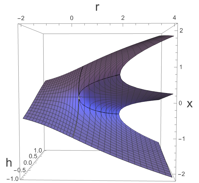
You should be able to rotate the figure to see it from all angles. Note that here we haven’t said what is a stable and what is an unstable fixed point. Do you notice anything familiar?

There is a lot going on here! Don’t worry if this isn ’t making sense at all yet.

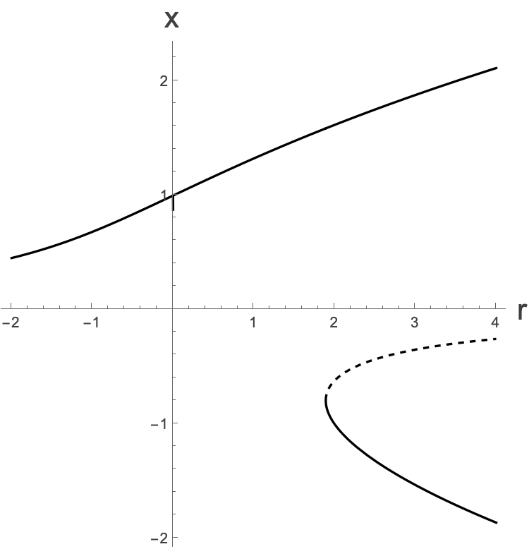
Let’s do a bit of a sanity check here. Let ’s take a slice through here at, say $h=0$, and see what we have:

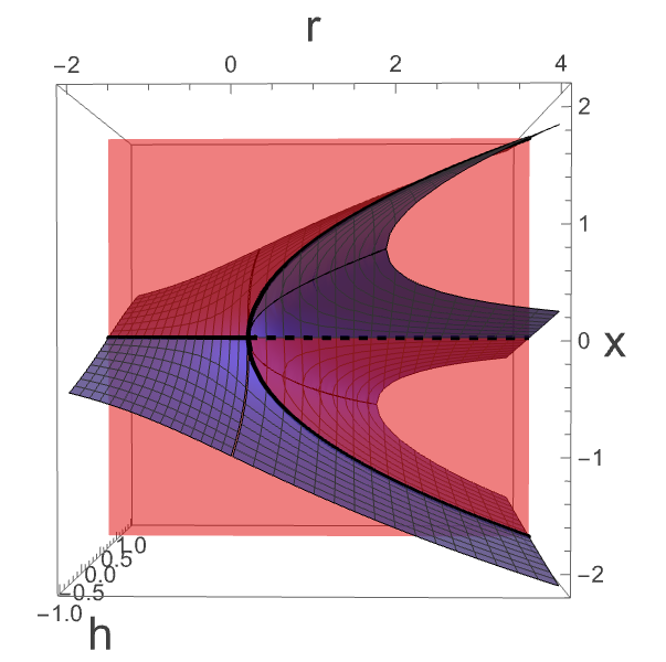
If you look at the intersection between the plane of $h=0$ and the surface that we’ve just created, you will see that it gives the plot for $h=0$ we’ve seen before. (Make sure you rotate if you can ’t see it)

And if we look at $h$ close to -1?

or $h=1$:

This strange surface that we’ve plotted looks a bit like a folded piece of cloth. Let’s look at a clearer drawing of it, taken from Steven Strogatz’s book on Nonlinear Dynamics and Chaos:

We need to dissect this a bit. What have we got here? So, for any given value of the parameters $h$ and $r$ (which correspond to things that we might be able to tune in our environment), we have different fixed points.

This strange shape is known as a cusp catastrophe. Why should it be called a catastrophe? Well, the reason for that is really because we can ask what happens if we have, for instance, $h=1$and we change $r$. Let’s plot that slice again:

Imagine that we have our parameter at, say $r=3$, and we are sat happily at our stable fixed point of around $x=-1.5$. Now let’s say something changes in the environment to decrease $r. $At $r=2$ our fixed point has moved to around $x=-0.9$. But then as we drop below $r=2$, our fixed point just…. vanishes. And all of a sudden we must move to the only fixed point in town, which is at around $x=1.6$. Let’s plot this…

Something very interesting happens here if we want to move back in the other direction!

What happens if now you start to increase $r$ again? Well, you will actually find that you stick on the upper branch. You won’t suddenly jump back.

This means that if the parameter changes even a tiny bit, you may well find that you are never able to get back to the situation that you were in before!

In fact the easiest way to see what is going on here is in terms of a potential (See Plot Below). Imagine that you are sat at the bottom of the stable minimum on the left, and you decrease $r$, from $r=2.6$ down to a little less than $r=0$ and then up again. You will find that as you pass $r=2$, you will go into the situation where there is only one minimum, and then as you increase r again, you will stay in the right hand minimum. If you are then in that new minimum, it’s really hard to get out again… there’s a great big maximum sitting in your way.

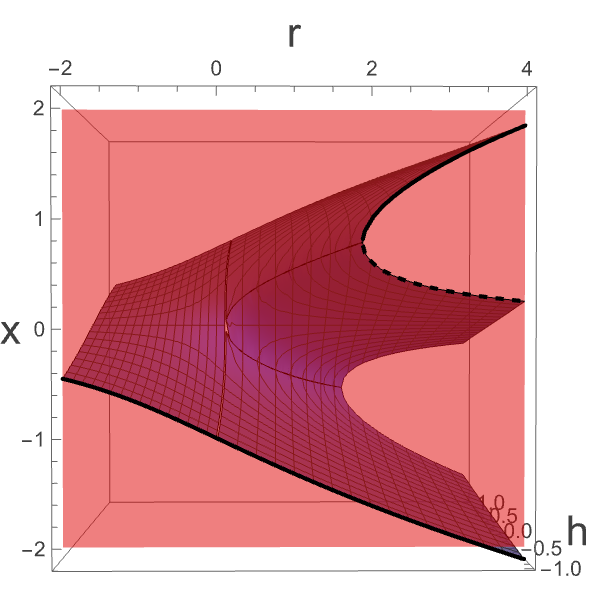
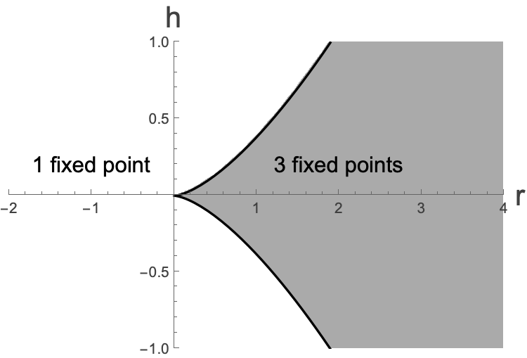
OK, there’s another way of plotting all of this. Let ’s look at the surface from above:

What do we see here? Well, we can see that for $r<0$, there is only ever one surface (i.e. one fixed point). It’s only as $r\geq 0$ that we start to get this “fold”, at which point we immediately have either one or three critical points, but it depends on the value of $h$. You can kind of see where this is in the ($r$, $h$) plane, but let’s plot it explicitly:

Exercise: One can model the population of insects by:

$$ \dot{N}=R N\left(1-\frac{N}{K}\right)-\frac{B N^{2}}{A^{2}+N^{2}} $$

Which has four free parameters, R, k, B and A, and N is the population of insects. It’s possible to convert this into an expression involving only non-dimensional variables, which can be written as:

$$ \dot{x}=r x \left(1-\frac{x}{k}\right)-\frac{x^{ 2}}{1+x^{ 2}} $$

which is now a differential equation with just two free parameters. See how far you can get in showing that this also has a cusp catastrophe.

There is a nice explanation of this example here but I’d like you to have a go at it yourself first. Have a watch of it, and see if you can understand the behaviour as you change the different parameters. In particular look at around 25 minutes to see the change as you slowly increase the reproductive rate of the population and how an insect outbreak can suddenly occur.