3.6 Chaos and the Logistic Map
Section 3.6: An Aside - Chaos and the Logistic Map.
Chaos and the Logistic Map
Let’s take a bit of a break from these bifurcations of first order differential equations and look at another situation where we get some very very interesting behaviour with fixed points. I’ve mentioned it briefly before, but let ’s go into some more detail. We’re going to be looking at not a differential equation, but a difference equation. This one is called The Logistic Map:
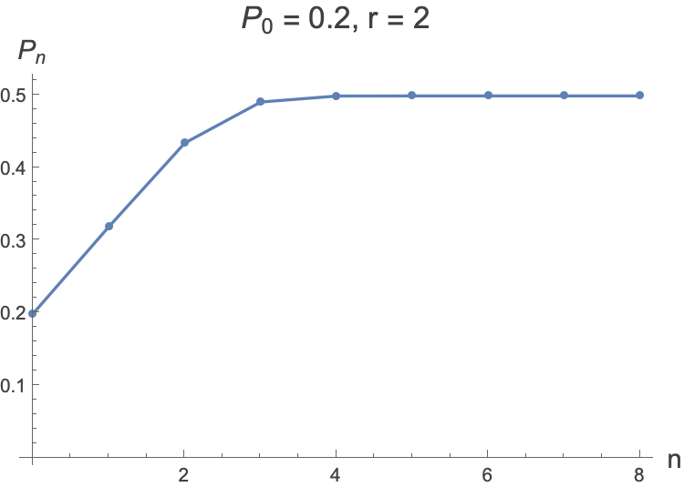
$$ P_{n}=r P_{n-1}\left(1-P_{n-1}\right) $$We can think of this as a population on a given day (or week, or year, or whatever), and $r$ is some sort of growth rate. It is related to the population at the previous time step. Let’s say $r=2$, if the population at time-step 0 is 0.2, then on the next time step, the population will be:
$$ P_{1}=2 0.2 \left(1-0.2\right)=0.4 0.8=0.32 $$So the population has grown. How about the next time step?
$$ P_{2}=2 0.32\left(1-0.32\right)=0.4352` $$We can write a piece of code which calculates the population through time for a given initial population and value of $r$ :
Let’s look at it with, a higher starting population:
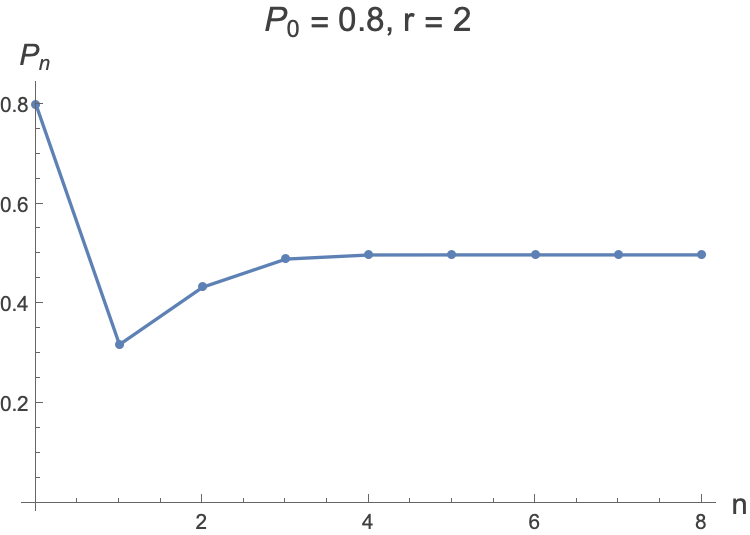
We see that starting at 0.8, the population first plummets, then it starts to go up again.
Exercise: Try and code this up yourself in Python.
If we start even higher, then something funky happens:
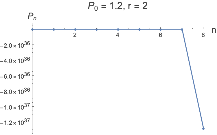
This looks bad! We seem to end up with a negative population. Well, while this doesn’t make sense in terms of a population, it still makes sense in terms of the equation. If we have a population greater than 1 at any time, then the next time step we will have a negative population, and once you have that, it will keep decreasing infinitely. So anything starting with a population of greater than 1 or less than 0 will end up flying off to -∞.
Let’s look at a range of starting values between 0 and 1:
We see that there are two fixed points here. One at 0, which is reached when you either start with $P_{0}=0,$ or $P_{0}=1$, and another one. A fixed point is defined by $P_{n}=P_{n-1}$ and so they can be found by solving:
$$ P_{n}=r P_{n}\left(1-P_{n}\right) $$Re-arranging this gives us:
$$ P_{n}=0 \text{ and } P_{n}=\frac{r-1}{r} $$which for the case of $r=2$ gives 0 and 0.5. What happens as we decrease $r$?
For $r=1.5$ the second fixed point seems to have moved down a bit. Let’s see what happens as we continue to alter $r$ :
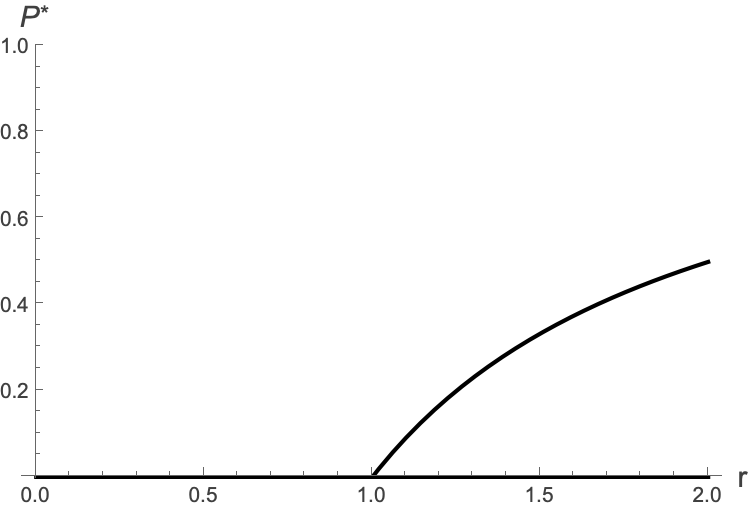
For $r\leq 1$, there is only one fixed point, and it’s at $P=0$. For $r>1$ there is a second fixed point at $\frac{r-1}{r}$.
We can plot the fixed points as a function of $r$ :
How on Earth could we find anything interesting in the humble Logistic Map equation?
Something strange is about to happen…
Let’s do our plot, but this time for, say $r=3.1$ with a starting population of $P=0.5$
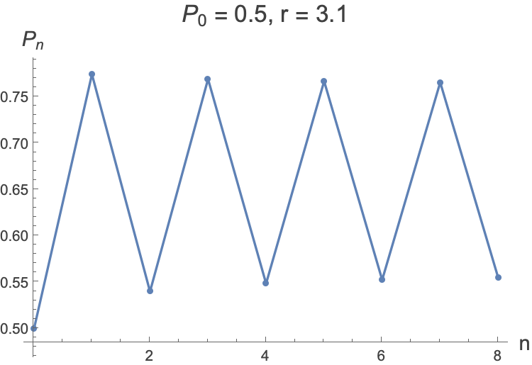
Wait a minute! It’s now bouncing between two values… it’s not the same as a fixed point, but there is a stable solution which includes just two values. This says that $P_{n}=P_{n-2}$. Can we figure out what these values are?
Let’s write down two equations:
$$ P_{n}=3.1 P_{n-1}\left(1-P_{n-1}\right) $$$$ P_{n-1}=3.1 P_{n-2}\left(1-P_{n-2}\right) $$but because $P_{n}=P_{n-2}$, we can write:
$$ P_{n}=3.1 P_{n-1}\left(1-P_{n-1}\right) $$$$ P_{n-1}=3.1 P_{n}\left(1-P_{n}\right) $$So here we have a set of coupled equation. Substituting $P_{n-1}$into the first equation we get:
$$ P_{n}=3.1 \left(3.1 P_{n}\left(1-P_{n}\right)\right)\left(1-\left(3.1 P_{n}\left(1-P_{n}\right)\right)\right) $$This has four solutions:
$$ P_{n}=0, P_{n}= 0.558, P_{n} = 0.677, P_{n}=0.765 $$It looks like we’re somehow bouncing between 0.558 and 0.765 in the above example. If we started at a higher value of $P_{0}$ we get
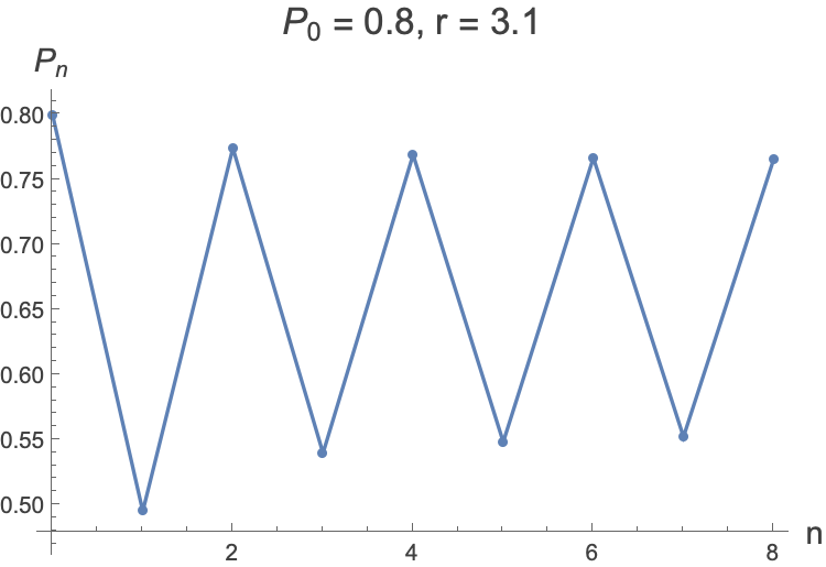
So where is that $P_{n}$=0.677 coming from? Well, that’s actually the true fixed point which never varies…but it’s unstable. Start anywhere away from it and you will end up bounding between these two values of 0.558 and 0.765.
Explore what happens if you start close to the true, but unstable fixed point.
Things are getting a bit complicated. We’re going to stick with an initial population of 0.5 from now on. Let’s write some code which outputs the late time behaviour…which will tell us which values it is bouncing between for a given value of $r$:
We can plot this now as a function of $r$:
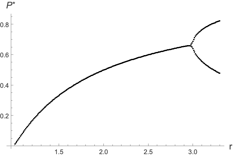
Note that $P^{*}$ shouldn’t be thought of as a fixed point, but one of a finite number of points which are jumped between.
So this says that for $r$ less than 3, you will reach a fixed point and stay there, but for $r>3$ you will find two points that you jump between.
Does anything else happen if we increase $r$ some more? Let’s look at the behaviour at $r=3.5$…
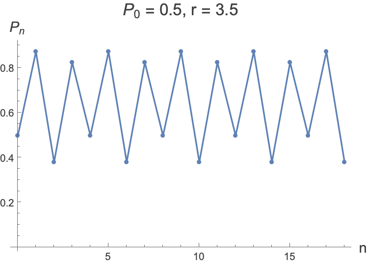
Hang on! Now we seem to be jumping between four values…let’s extend our $P^{*}$plot and see if we can see this.
This going from one to two to four values that we jump between is known as period doubling.
Well I never! We seem to have split once more… and if we continue, will we just keep doubling? I’m going to plot only from $r=2.5$ upwards.
What the…!?!? Has something gone wrong with our program?
Something completely weird seems to be going on… We found that we bounced between two stable points, then four, but now what on Earth is happening? Let’s look at, say $r=3.65$:
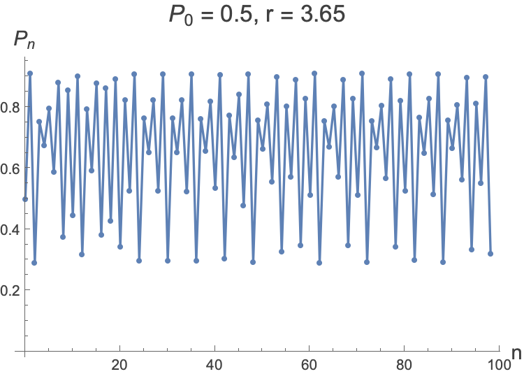
We seem to be jumping all over the place, however there is some structure in here. What if we look at $r=3.7$. Surely it’s going to be basically the same, no?
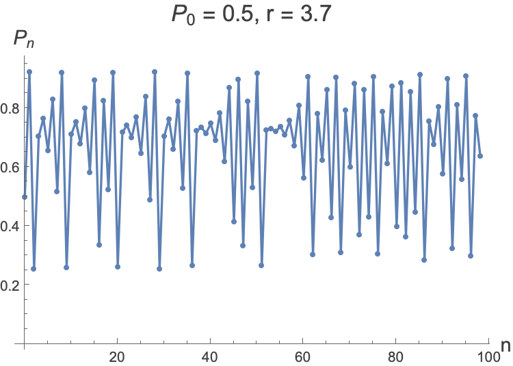
That seems pretty different… Let’s actually zoom into a region between 3.6 and 3.61…
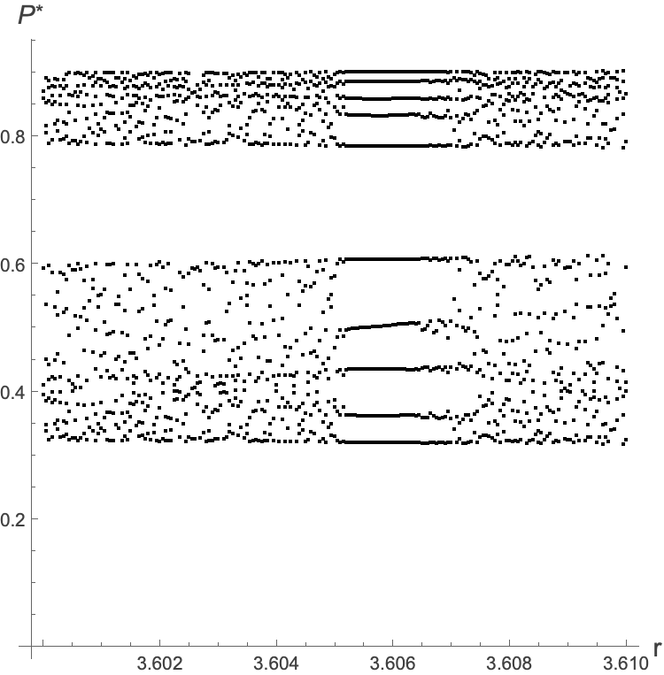
You can see that this seems to be chaotic… and indeed that’s exactly what it is!! If you change the value of $r$ just slightly, the behaviour changes a huge amount. This sensitivity to the parameters is called chaos.
The strange thing is that within this chaos we see an island of calm, between around 3.605 and 3.6065. And indeed within the chaos you will keep seeing islands of calm.
Exercise: Explore this with Python.
What has this got to do with the real world? Well, it turns out that a lot if not most of what is around you is part of a chaotic system!
You can look at the times that the period doubling occurs, and see how much you need to increase $r$ by until the next one. It turns out that if you take the ratio of these period doubling times you get a constant related to this, called δ, the Feigenbaum constant which is:
$$ \delta{}=4.669... $$and this number appears all over nature in systems that become chaotic.
Mathemafrica: Mandelbrot set.
Have a look at this blog-post:
to learn more about Feigenbaum and his constant.
If you haven’t already done so, take a look at the Veritasium video on this here .
I’m going to leave you with this interactive plot. See if you can figure out what’s going on. The red dashed line is a line of gradient 1 through the origin (the diagonal $P_n = P_{n-1}$). The blue parabola is $P_n = r\,P_{n-1}\,(1-P_{n-1})$. The green cobweb starts at $(P_0, 0)$ and bounces between the parabola and the diagonal — each pair of edges is one iteration of the map.
Back to our study of first order differential equations!