3.5 Combinations of Bifurcations

Section 3.5: Combinations of Bifurcations

Combinations of Bifurcations

Let’s look at a bit more complicated system:

$$ \dot{x}=r x+x^{ 3}-x^{ 5} $$

This is similar to the subcritical pitchfork bifurcation, but now with an extra $x^{ 5}$ term. Let’s start by looking at the roots of the right hand side (which of course correspond to the fixed points). It ’s messy, but it’s possible to show that this has zeros/fixed points at:

$$ x=0, x=\sqrt{\frac{1}{2}\left(1-\sqrt{1+4r}\right)}, x=-\sqrt{\frac{1}{2}\left(1-\sqrt{1+4r}\right)}, x=\sqrt{\frac{1}{2}\left(1+\sqrt{1+4r}\right)}, x=-\sqrt{\frac{1}{2}\left(1+\sqrt{1+4r}\right)} $$

So we have five different zeros. However, for a given value of $r$, not all of these give us real numbers. For instance, for $r<-\frac{1}{4}$, we can see that all of the terms with square roots are undefined, so for this region of $r$ there will actually only be one fixed point. The bifurcation diagram is found by plotting all of these functions of $r$. We will check the stability of the points in a bit…

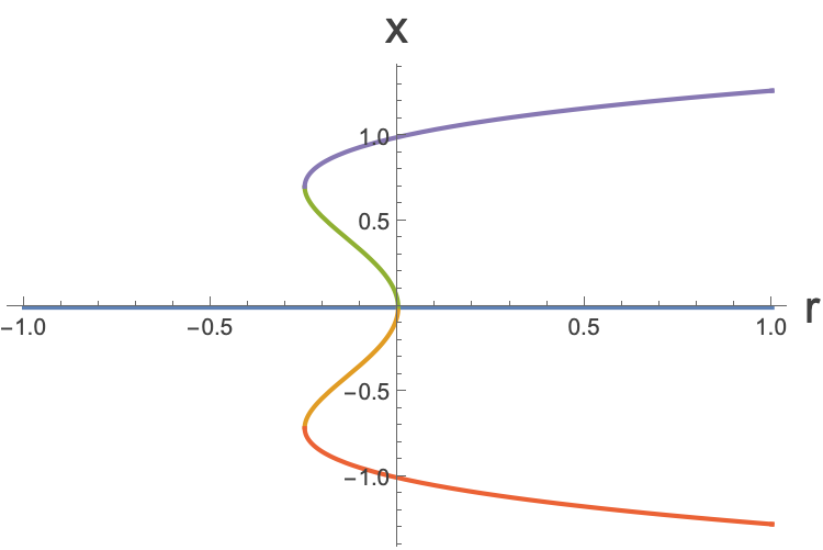
Each color corresponds to one of the above roots of the equation

$$ r x+x^{ 3}-x^{ 5}=0 $$

ok, so we can see that we have changes in behaviour at $r=-\frac{1}{4}$ and $r=0$. Let’s explore the phase portraits for the different regions. We’ll skip the fixed points at first and just plot the $\dot{x}$. We will plot it for $r=-\frac{1}{2}$ (below the first bifurcation point), at $r=-\frac{1}{4}$ (at the first bifurcation point), at $r=-\frac{1}{8}$ (in between the first and second bifurcation point), at $r=0$ (at the second bifurcation point) and at $r=\frac{1}{2}$(above the second bifurcation point).

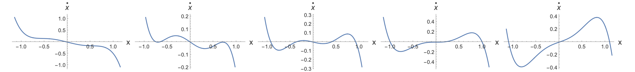
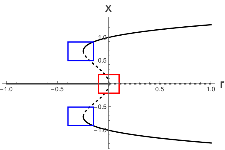
As an exercise, draw on the fixed points and whether they are stable or unstable. From this, you should be able to get the following bifurcation plot:

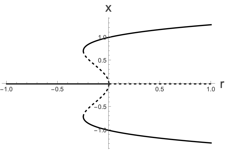
Notice that we have two saddle-node bifurcations appearing at $r=-\frac{1}{4}$, and then a subcritical pitchfork bifurcation happening at $r=0$. Let’s just box these to make sure that it ’s clear. The saddle-node bifurcations are in blue, the pitchfork is in red.

Now check the type of fixed points you drew on the phase portraits.

Let’s step back for a moment and try and get a bigger picture… this has gotten pretty messy!

We started here with a differential equation which may describe the dynamics of some physical system. We want to know some of the qualitative features of the behaviour of this system. One of the most important types of qualitative thing we can talk about are the fixed points, and their nature. We have a parameter, $r$ and we know that for different values of this parameter there may be different numbers of fixed points. We figured out where the fixed points were, and you figured out what kinds of fixed points they were. Of course one can run the linear stability analysis on the fixed points and see whether they are exponential, or less than exponential in their behaviour.

Hysteresis

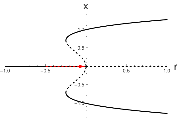
Let’s ask now, not just about where the fixed points are, but how you might move around them. Let’s say you start your system off with an $r$ value (which you can tune by a dial on your equipment) of $r=-0.5$, and an $x$ value of $x_{o}=0.1$. Close to $x=0$ you can do a linear stability analysis and show that the equation looks like:

$$ \dot{x}\approx{}r x $$

Which means that we will have a behaviour with these parameters of:

$$ x=0.1 e^{-0.5t}. $$

So we are getting closer and closer to $x=0$ over time.

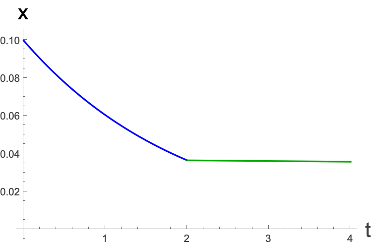
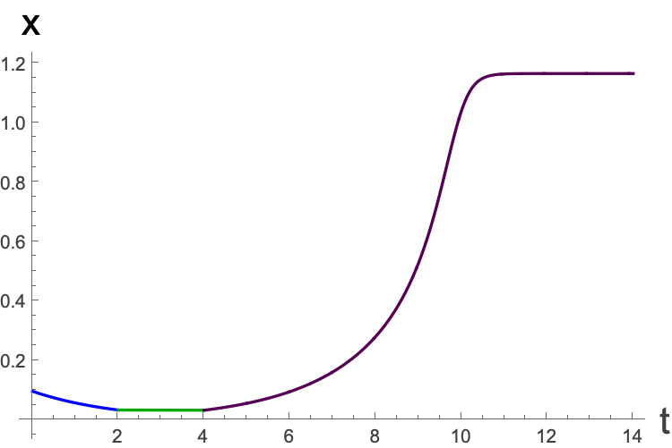
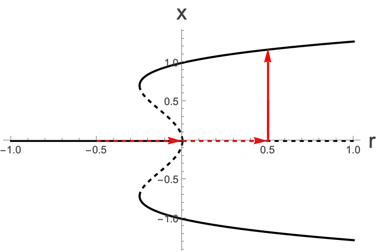
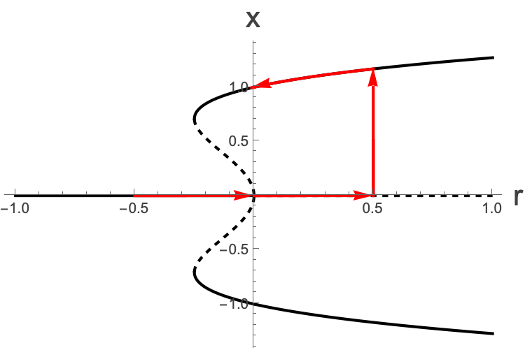
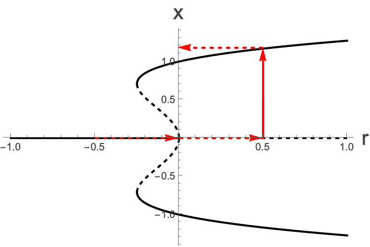
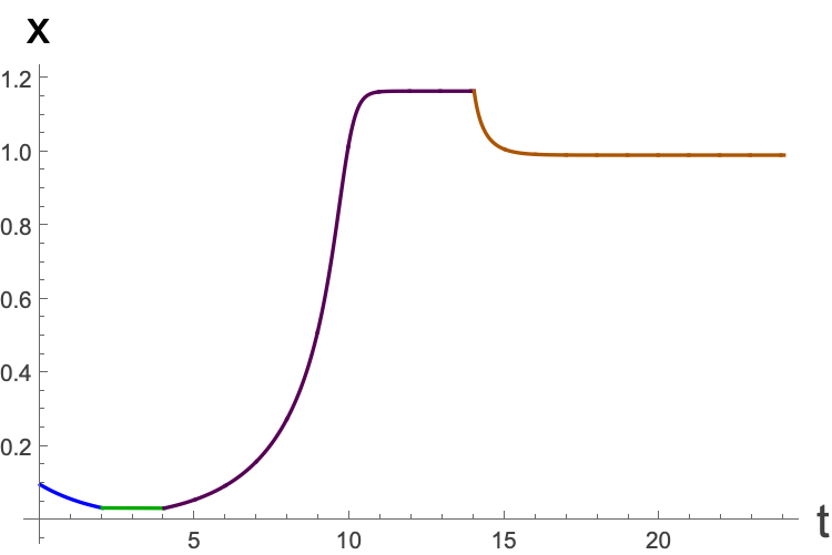
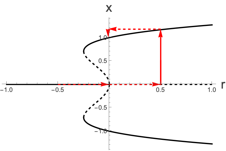
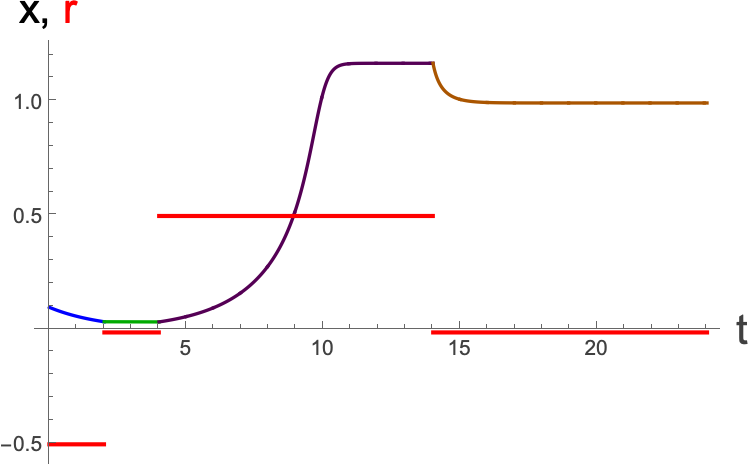
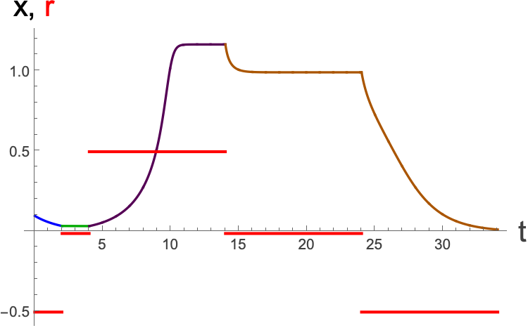
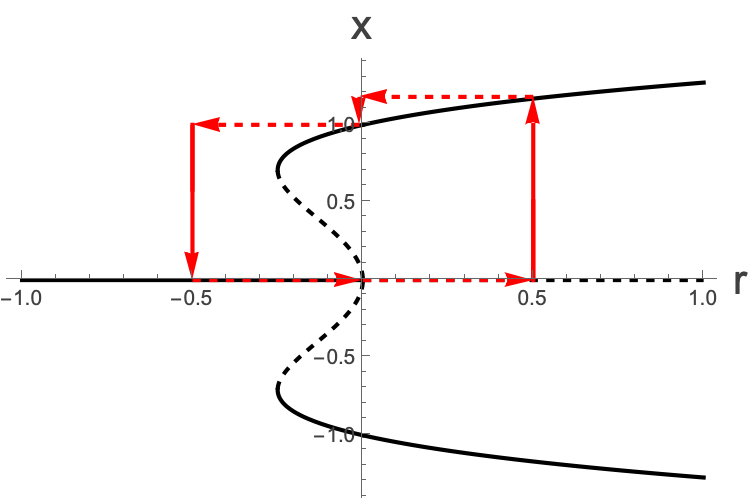
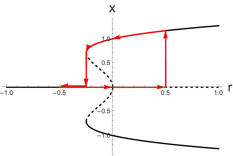
Let’s say that we now quickly increase our value of $r$ to $r=-0.01$. Because we are close to $x=0$, the linear stability analysis around here remains the same and so we will remain close to $x=0$. Notice that for values of $\frac{-1}{4}

Because of our exponential decay, we are still at a positive (though small) value of $x$. It actually depends how quickly we move our dial and how long we ’ve been waiting as to how small, but we know that we couldn ’t have crossed over to a negative value of $x$. Let’s say that after waiting at $r=-0.5$ for 2 seconds, we suddenly altered the value of $r$ to -0.01 and stay there for 2 seconds. We can first work out that after the first 2 seconds our $x$ value would be:

$$ x\left(2\right)=0.1 e^{-0.5 2}=0.1 e^{-1}=0.0367879441171 $$

Then our new r value is -0.01 and we wait there for 2 seconds:

$$ x\left(4\right)=0.036787944117144235` e^{-0.01 \left(4-2\right)}=0.0360594940173 $$

Let’s think careful about where that $\left(4-2\right)$ comes from. The solution to the new equation is:

$$ x=x_{o} e^{-0.01t} $$

but we started now not at $t=0$, but really at $t=2$, so everything should be measured from $t=2$. The amount of time that we have been sat there at $t=4$ is 2 seconds in the new $r=-0.01$ system, and the initial condition is the value that we were at the end of the $r=-0.5$ system, which was 0.0367879.

In terms of the trajectory, this looks like:

Note that in seconds 2 to 4, it looks flat but we are still decaying, just with a decay rate of only $-0.01$

Now let’s say that we move our dial to $r=0.5$. Suddenly the value of $x$ that we are sitting at is an unstable fixed point. In fact we will move away from it now with an exponential of the form:

$$ x=x_{o} e^{0.5t} $$

Where our $x_0$ is 0.0360595. Of course we can only trust this behaviour when we are close to the unstable fixed point, and really we would have to solve the whole system, so we ’ll do that numerically with Euler’s method with a step size of 0.01 for 1000 steps and see where we get to:

This takes us to 14 seconds and to an $x$-value of 1.16877:

On the bifurcation diagram it looks like we have made this journey:

[ Dashed arrows are instantaneous jumps in $r$, the full red arrows are trajectories which take time to get to a new x value ]

ok, so what happens if we now move the value of $r$ back to -0.01?

We could do this by either slowly tuning r down, in which case it’s going to stick to the positive stable fixed point:

Or we could suddenly shift $r$ to $-0.01$ , in which case for a moment, the value of $x$ would be away from the new fixed point:

We will do this, and then “wait for a couple of seconds” and see what the trajectory looks like. We can again use Euler’s method, now starting with $t=14, x=1.16877$:

Then we find ourself at the upper fixed point again:

Let’s just add to this the values of $r$ across time as well. These are in red:

Now, if we suddenly change the value of $r$ back to the original value of $ r=-0.5$, we will get:

Which corresponds to: (We can see it goes to the nearest stable fixed point in that vertical slice!)

So what is the conclusion here, and what of the word hysteresis?

Well, we have started with $r=-0.5, $gone up to $r=0.5$ and then come back down again, and yet the values of $x$ hasn’t just stayed close to the $x=0 $fixed point. It’s taken us on a whole loop. We were at $r=-0.01 \text{ twice and }$ each time we were at a different value of $x$. Hysteresis is about the system knowing where it has come from in order to know the state.

You could have done the above, but changed the value of $r$ slowly, in which case you would have:

Here we can see it all together, with a dial for $r$ on the left, the trajectory in the ($t$, $x$) in the middle, and the trajectory around the bifurcation plot on the right.

Here is a really strange example of hysteresis: If you take water at room temperature and freeze it, it will take a certain amount of time to freeze. However, if you boil water, and then freeze it, it actually freezes faster, despite the fact that in order to freeze, it has to pass through the room temperature state.

There is information in the system about what happened to it in the past (you can think of it as remembering that it was in a high temperature state - though note very very importantly, this “memory” is not like the memory which people claim that water has in homeopathy. That isn’t memory, it’s wishful thinking). This phenomenon with water is called the Mpemba Effect , named after the Tanzanian schoolboy who discovered it. It’s actually not completely agreed upon what is the cause of this effect.

That was a lot! We’re going to look at something a bit different on the next page before returning to the study of these bifurcations.