3.1 & 3.2 Introduction and Saddle-Node Bifurcations

Section 3.1: Introduction to Bifurcations

Introduction to Bifurcations

Let’s say I gave you the differential equation:

$$ \dot{x}=x^{2}+r $$

and asked you to find the fixed points. You would, quite rightly, tell me that I haven’t given you enough information. It should certainly depend on the value of $r$ as to where the fixed points are… or indeed if there are any at all!

Luckily we can study the system for different values of $r$ and see if you can explore patterns in the fixed points.

One way to think of this would be if you had an equation which described some physical system, and there was a free parameter (a growth rate, a carrying capacity, a friction term, an external magnetic field etc.) and you wanted to know how the system would change as you altered this parameter. A non-free parameter is a parameter that can’t take on different values e.g.) Planck’s constant, or the speed of light.

It turns out that fixed points can change qualitatively. They can appear, or disappear, in a variety of interesting ways. And that is what the study of bifurcations is going to be. Bifurcation points are the points where the fixed points of a system alter in number, or in type.

An often-cited example is a vertical beam which can support some weight. If the weight is small, then the beam is stable. However, if you increase the weight, the beam will buckle. This will typically happen after some critical weight is added.

Saddle Node Bifurcations

The equation that we wrote above:

$$ \dot{x}=x^{2}+r $$

is the one that we want to study to start with. Here are four phase portraits which correspond to different values of $r$ in the above equation.

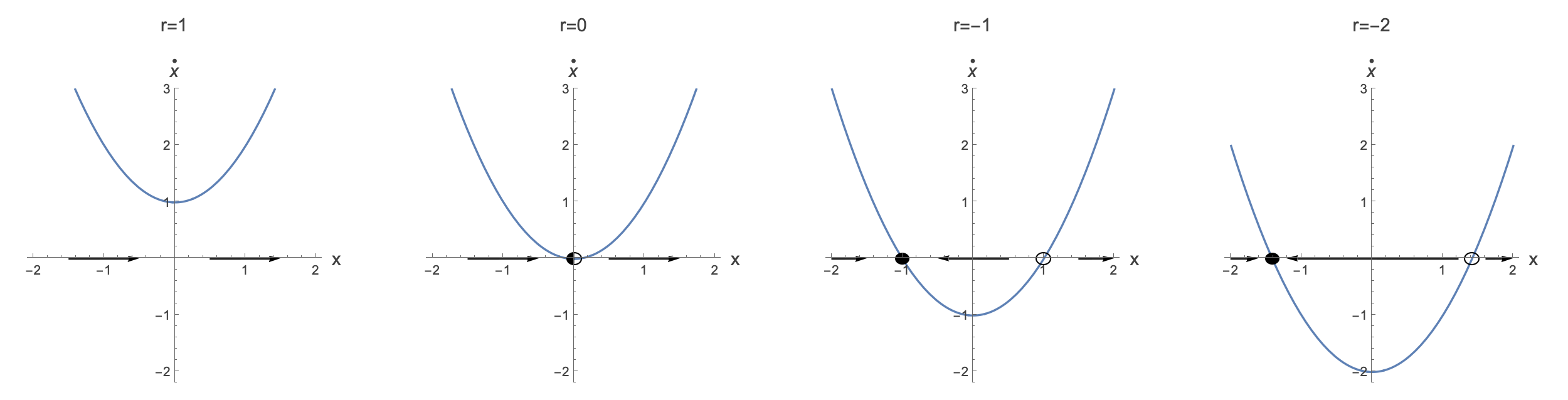
We see that as we change the value of $r$ we go from no fixed points if $r=1$, to one semi-stable fixed point at $r=0$ to a stable and an unstable fixed point at $r=-1$ which get further apart as you make $r$ even more negative.

Well, how about plotting the positions of the fixed points at different $r$ values? We can do this, and include the arrows in what is called a vector field:

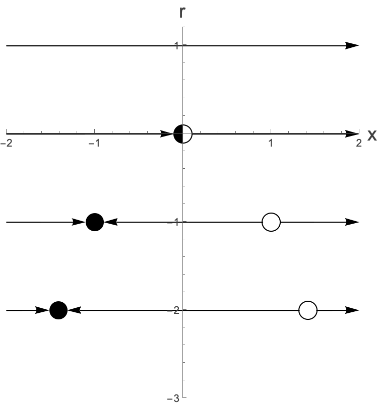
Now notice how we’ve shown the position of the fixed points in relation to different values of $r$.

In fact, we can also exclude the arrows, and just put in the fixed points using solid lines for stable fixed points and dashed lines for unstable fixed points. Usually this is done by taking the above diagram and putting it on its side, so the $x$ direction is vertical.

Clearly the fixed points are the values for which $\dot{x}=0$ which in this case is just the roots of $x^{2}+r$. So we just have to solve for x as a function of r and get an expression!

$$ x^{2}+r=0 $$

Clearly for $r\leq 0$ this is just $x^{*}=\pm{}\sqrt{-r}$. This will look like:

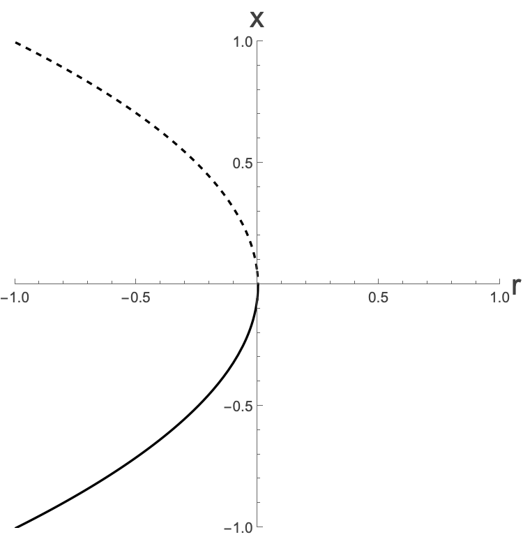
This is known as a Bifurcation diagram. [Note the Independent Variable on the Horizontal Axis]

Where note that the $x$-axis has become the vertical axis because what we are plotting here is the position of the fixed points as a function of the parameter $r$. The dashed line corresponds to unstable fixed points, and the full line is the stable fixed points. To understand this plot, choose an $r$ value (say $r=-0.2$) and imagine taking a vertical slice at that value. You will see that the line will cross two fixed points like so:

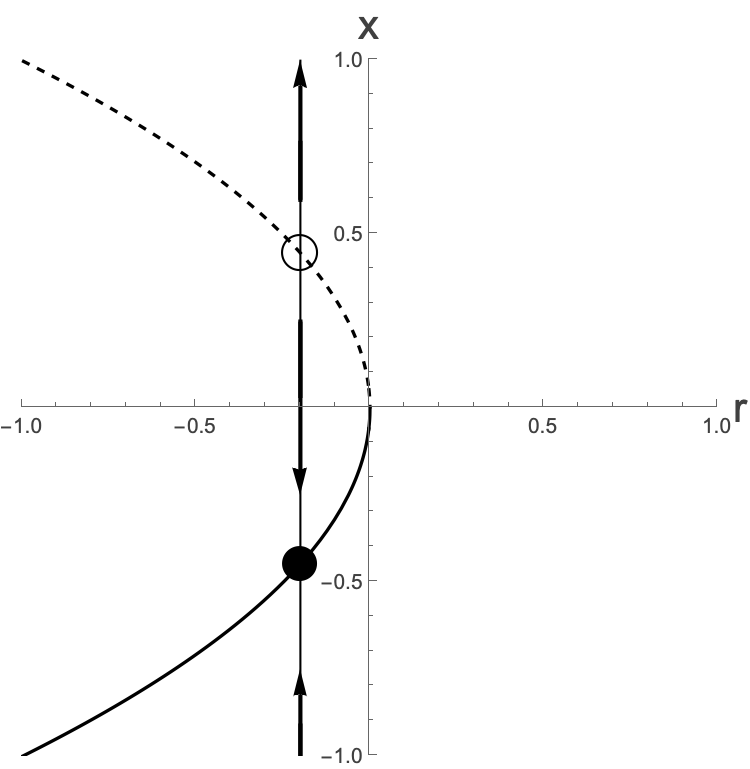
Now this slice is just the flow line you all know and love, if you tilt your head to the left.

So, this bifurcation diagram gives us a summary not just of the fixed points of a single equation, but of a whole family of them, as we change some parameter.

This particular type of bifurcation where two fixed points come together (at $r=0$) and are ‘destroyed’ is called a saddle-node bifurcation. You can imagine that as you increase $r$ from negative values towards zero, two fixed points ‘collide’ and annihilate with one another, leaving no fixed point at all after this point. The bifurcation happens at $r$ = 0. The point at which this happens is called the critical point, and in this case we would write $r_{c}=0$.

Note that this bifurcation type is also sometimes called a fold bifurcation or a blue sky bifurcation (two fixed points appearing out of the blue).

Note that the fixed points can come together from the left, or right (increasing or decreasing $r$), and meet at any point, but the thing which makes a saddle node bifurcation a saddle node bifurcation is that when you change a parameter you go from two fixed points to zero.

The term bifurcation has its origins in the idea of turning into two forks (bi=two, furc*=fork, from Latin)*.

Now your turn: Perform the same analysis as above, but this time for the equations:

$$ \dot{x}=r-{\left(x+1\right)}^{2} $$$$ \dot{x}=r-x+e^{ x} $$

The coming few pages are going to be about classifying the other types of bifurcations. But before clicking through, see if you can picture what they might be.

Actually, let’s run through the second example above together. There are a few reasons that it will be very instructive.

The first thing to note is that this equation

$$ \dot{x}=r-x+e^{ x} $$

looks very different to the saddlenode bifurcation form that we first wrote down:

$$ \dot{x}=x^{2}+r $$

What we are going to show is that close to the bifurcation point, they are actually the same. It turns out that this is always true! If ever we have a stable and unstable fixed point appearing out of nowhere at a bifurcation point, we can ALWAYS perform a change of variables such that close to the bifurcation point our system looks like the above normal form of a saddlenode bifurcation.

First, let’s get a bit of intuition about the above system. The first thing that we can ask is where the fixed points are. This is clearly when $\dot{x}$=0, ie. when:

$$ 0=r-x^{*}+e^{ x^{*}} $$

Where we have indicated that these values of $x$ are fixed points. We would like to be able to plot the bifurcation diagram, which corresponds to writing the positions of the fixed point as a function of $r$. However, that would involve solving the above equation for $x^{*} \text{ which } $can’t be done. We can however write $r\left(x^{*}\right)$ rather trivially:

$$ r=x^{*}-e^{ x^{*}} $$

and plot this:

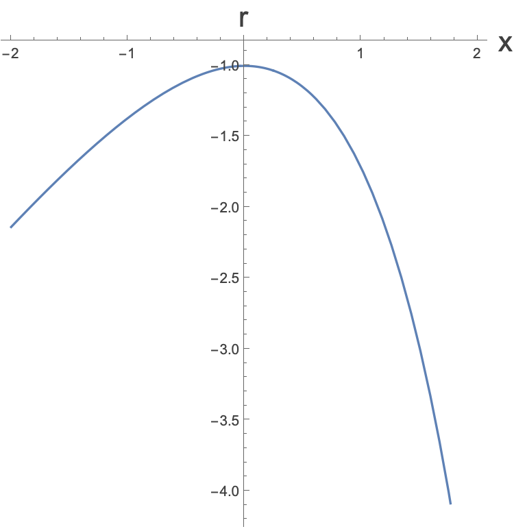
where here we generally write x on the axis rather than $x^{*} \text{ but }$ we should remember that we are here plotting the positions of the fixed points. We haven’t said anything here about the stability of the fixed points. To find this, we need to know the value of the derivative of $f\left(x\right) \text{ with respect }$ to $x$ at the fixed point. Given

$$ f\left(x\right)=r-x+e^{ x} $$

we have

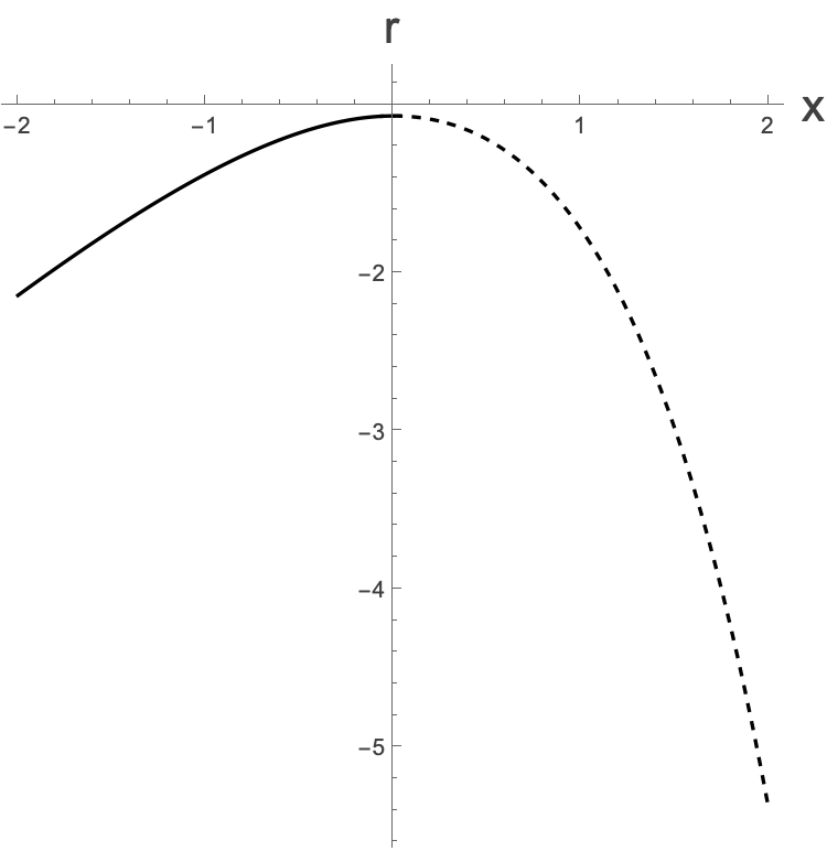
$$ f'\left(x\right)=-1+e^{ x} $$

which we can see is negative for $x<0, \text{ corresponding to } $a stable fixed point and positive for $x>0$, corresponding to an unstable fixed point. Making this clear on the graph above, we have:

For the bifurcation diagram, we need to flip the axes around here, which we can do graphically, even though you can’t actually calculate the inverse of $-x+e^{x}:$

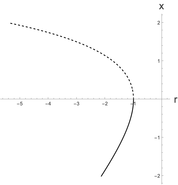
So this is our bifurcation diagram. We see that as we decrease $r$ the two fixed points suddenly appear at $r=-1$.

The claim is that the bifurcation point is the same as that of the original equation that we looked at. To see this, we are going to take our system, and expand it around $x=0$, which is where the bifurcation occurs in $x. Close \text{ to } x=0$, we have:

$$ \dot{x}\approx{}r-x+\left(1+x+\frac{x^{2}}{2}+...\right) $$

So close to $x=0, \text{ taking only } \text{ up to } \text{ the quadratic } \text{ term in } x \text{ we have }:$

$$ \dot{x}=r+1+\frac{x^{2}}{2} $$

ok, so this is looking a little more like the original equation, but we have an $r+1 \text{ and we } \text{ have } $a factor of 2 in the denominator. Let’s write this out as:

$$ \frac{d x}{d t}=r+1+\frac{x^{2}}{2} $$

let’s first try and get rid of the 2. We can make a change of variables $t=2T$ to some new time coordinate. Doing this and using the chain rule we get

$$ \frac{d x}{d t}=\frac{d T}{d t}\frac{d x}{d T}=\frac{1}{2}\frac{d x}{d T}=r+1+\frac{x^{2}}{2} $$

multiplying through by 2 we have

$$ \frac{d x}{d T}=2\left(r+1\right)+x^{2} $$

and now letting $2\left(r+1\right)=R$ we have:

$$ \frac{d x}{d T}=R+x^{2} $$

which is exactly the same form that we started with. It turns out that for all saddle-node bifurcations this is true. We can always make this change of variables to put our equation, close to the bifurcation point in the Normal Form.

What this tells us then is that if we study just the Normal Form equation, and all saddlenode bifurcations are really the same as the Normal Form saddlenode bifurcation close to the bifurcation, then we understand all saddlenode bifurcations, however strange they may look.