2.7a Solving Equations on the Computer

Section 2.7a: Solving Equations on the Computer

Solving Equations on the Computer

This course is about how to get as much out of your dynamical systems without having to solve any, or at least too many, differential equations.

Euler’s Method

Most of this is going to take the form of these geometrical methods that we’ve been describing - phase portraits, fixed points, stability analysis, and similar. We want to be able to get a computer to do the hard work for you. One of the simplest ways is so called Euler’s method, and it works particularly well for these single, first order differential equations. Let’s take a particular example we’ve seen before. The logistic equation:

$$ \dot{P}=P\left(1-P\right) $$

where we have chosen the growth rate and the carrying capacity both to be 1.

Let’s say we want to know what’s going to happen if we start with a population of 0.2 (i.e. $P\left(0\right)=0.2$). (let’s say that the units are in millions of… Hmmm… Rabbits). Let’s plot this point as the starting point of our trajectory:

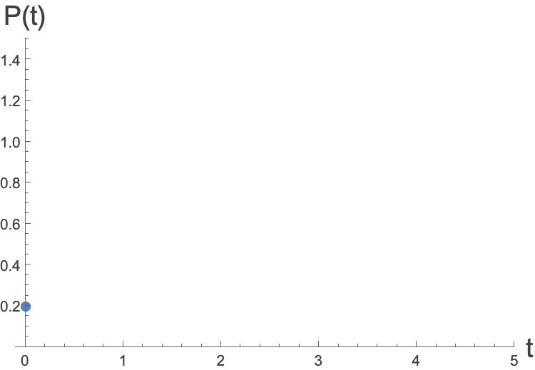
What would the rate of change of the population at this point by? Well we have an equation for that!

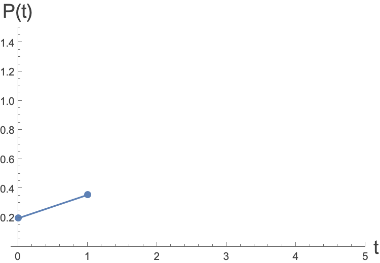
$$ \dot{P}=0.2\left(1-0.2\right)=0.16 $$

Clearly, if the population doesn’t change much, then the gradient isn’t going to change much. So let’s roll forward time with a rate of change of P of 0.16 for, let’s say 1 timestep. Where would this take us to? (Euler’s Method)

$$ P=0.2+0.16 1=0.36 $$

That’s now our new population. Let’s put that on our trajectory, and join the points:

Now we do the same thing again. Now we’re at $P = 0.36$, so what’s the rate of change now?

$$ \dot{P}=0.36\left(1-0.36\right)=0.2304 $$

The gradient has increased a bit. Let’s use this gradient and roll forward again for one time step:

$$ P=0.36+0.2304 1=0.5904 $$

Which gives us:

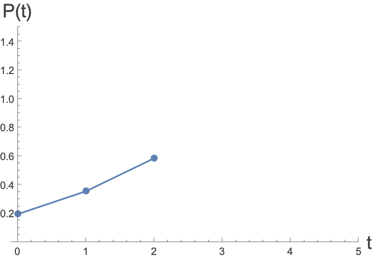
We can continue with this… Using a computer program we can automate this process. Let’s do this for another few steps:

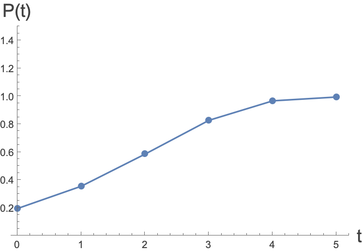
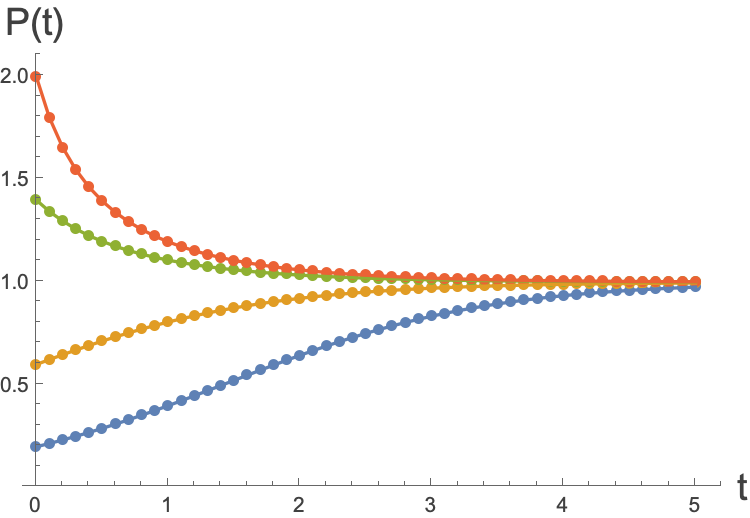
We see that it’s doing what we expect from a fixed point analysis. We know that $P=1$ is a fixed point, and we can see that we are gradually going towards this value.

The idea is to use the equation to approximate the gradient over the next short time step as the actual gradient at the start and moving in a straight line with that gradient through the interval and then repeat.

We could have taken smaller time steps which would be slightly more accurate. This is because the gradient of the smooth curve changes less over a smaller interval. Let’s go with time steps of 0.1:

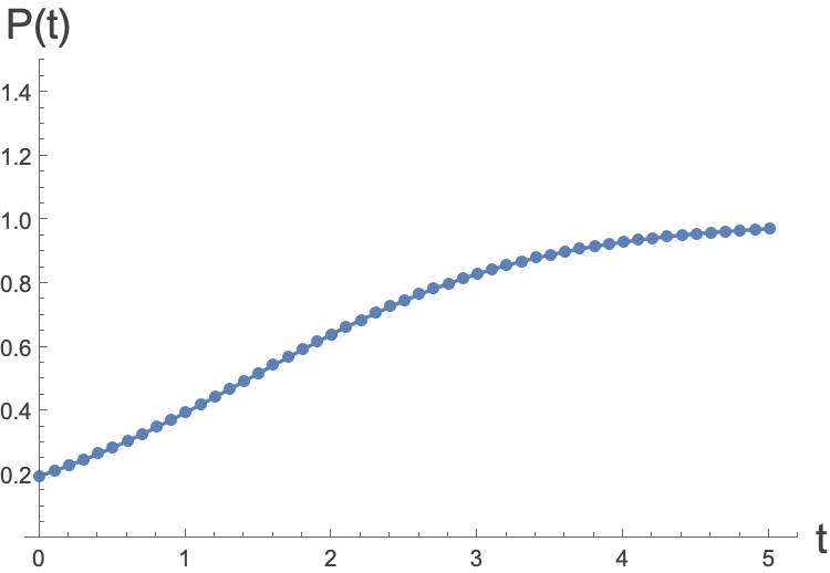
This is actually already very close to the exact solution and we didn’t have to do any integration! We can do the same thing for a range of different starting values of the population and we get this:

I’ve done this in Mathematica, but now you try and do this using your Python skills.

Euler’s method, is one of the simplest ways to explore these differential equations. One can do the same thing with higher order differential equations. In fact there are hundreds of books written on the subject of numerically solving differential equations, but we’re not going to explore that too much here.

Direction Fields

There is another computational method that we can use which is a so-called Direction Field. We’ll look at a non-autonomous differential equation, as it’s pretty simple, and you can see that it’s even simpler if the system is autonomous.

Let’s look at the equation:

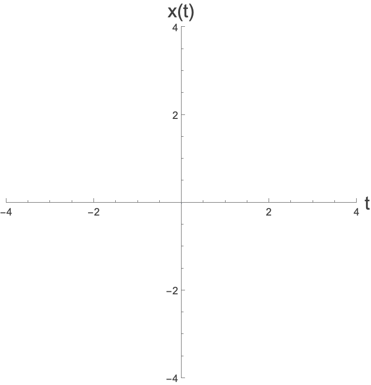
$$ \dot{x}=x+t $$

We see that this is non-autonomous because there is an explicit $t$ sat in there. This tells us that the rate of change of $x$ is related to the value of $x$ and $t$ very simply. Let’s plot the $\left(t,x\right) $plane, which is where we can see trajectories. Let’s plot it for $t$ in the range [-4,4] though we could have chose anything, and let’s choose $x$ in the range [-4,4] as well.

There’s no trajectory in here yet, but let ’s see. Let’s ask what the trajectory would look like at $t=0$. Well, according to the differential equation, that would depend on the value of $x$. For instance, at $t=0$, if you are at the point $x=1$, you will have a gradient in the $\left(t,x\right) $of:

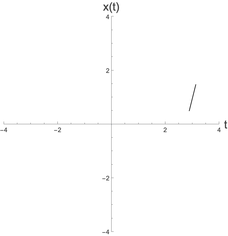
$$ \dot{x}=1+0=1 $$

So, what we are going to do is draw in a short line segment, let’s say of length 1 at this point, with gradient 1.

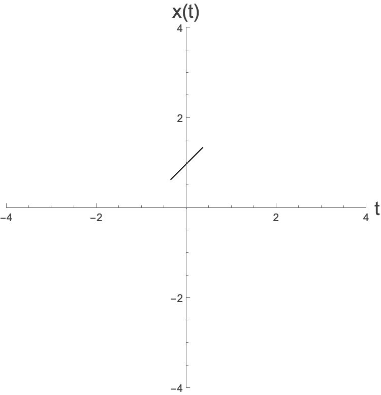
The idea here is that if you knew the true trajectory, as it passed through the point (0,1) it would look something like this. We can do the same thing at lots of other points in the plane. For instance, at the point (3,1), we would get a short line of gradient 4 which would look like:

Now let’s do this all over the plane:

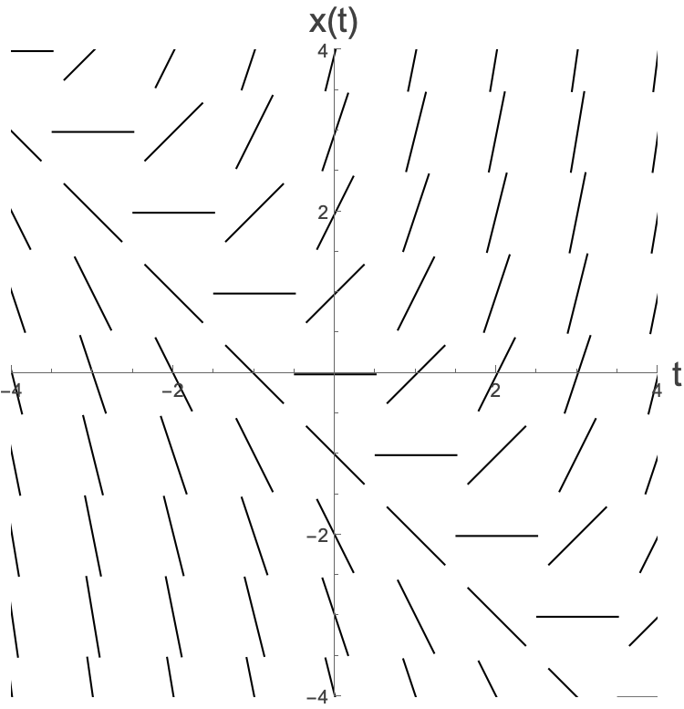
Let’s do it for more points, and with slightly shorter lines:

We can picture this like looking at a stream, where you have dropped a little bit of coloured dye into many points, and are watching the flow. You can imagine that you start at some point, move along that line, then find the nearest next line, and follow that, etc. This gives you a trajectory.

These lines are known as direction fields and are another way of figuring out the behaviour without actually having to solve the differential equation.

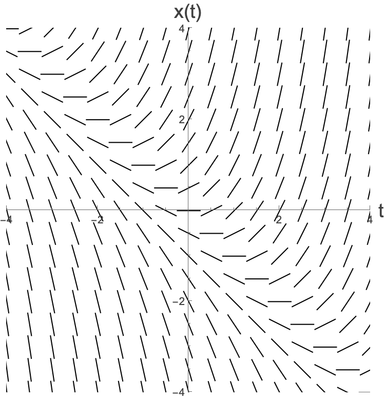
As I said, this is for a non-autonomous system. Had we gone with an autonomous system, let’s say

$$ \dot{x}=x $$

Our direction field would look like this:

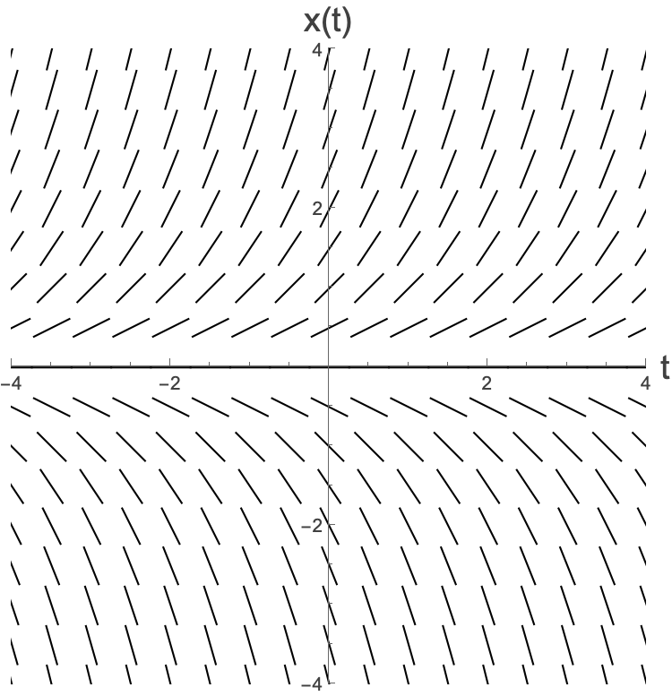
Which is a perfectly good direction field, but we notice that the gradients of the lines have nothing to do with the value of $t$ as we would expect from the equation. We can spot here the fixed point of $x=0$, and indeed note that it is an unstable fixed point. You will always flow away from it.

Soon we will move on to section 3 and explore bifurcations, which is really about the way the fixed points can themselves behave. First of all, let’s have a quick recap of phase spaces and phase portraits.