2.1 Fixed Points and Trajectories
Section 2.1: Fixed Points and Trajectories
Flows on the Line - Fixed Points and Trajectories
We’re actually going to focus on the simplest system of differential equations - a single differential equation. We’re going to see what interesting discoveries we can make in such simple settings. For this chapter we will be dealing with equations of the form:
$$ \dot{x}=f\left(x\right) $$Please note:
We use $\dot{x}$ as the shorthand for $\frac{d x}{\text{ dt }}$
We leave out the functional dependence on t (i.e. write $x$ rather than $x$(t) most of the time)
Recall, we can have equations where $f$ is itself a function of $x$ and $t$ explicitly ( $\dot{x}=x+t^{2}$), but these non-autonomous systems can always be rewritten as autonomous systems of one more equation (we won’t be dealing with these).
Here, $x $is a function: (For our purposes it’s always going to be differentiable)
$$ x:\mathbb{R}\longrightarrow{}\mathbb{R} $$This is an equation on a line, or a flow on a line, because you can imagine that $x$ is the position (let’s say of a particle) on a line at time t, and the dynamical equation tells you how you move along the line. In particular, your velocity (which is just $\dot{x}$ ) at any particular position (velocity is change in displacement, x, over time).
We’re going to start with an example that is possible to solve exactly, but we’ll see that we can get a lot out of it without doing so.
Our first equation is:
$$ \dot{x}=\text{ sin }\left(x\right) $$Think of our particle on a line, and this just tells us that the velocity along the line at any one point is given by the sin of that point’s position.
It is actually possible to solve this, but it is a pain… and we can be lazy. I’ll write out the solution, but you don’t need to know this!!
$$ x=2 {\text{ cot }}^{-1}\left(e^{-t}\text{ cot }\left(\frac{x_{0}}{2}\right)\right)+2\pi{} n\left(x_{0}\right) $$where $x_{0} $is the position at time $x=0$, and we have a function $n\left(x_{0}\right)$ which we won’t go into, but it’s always an integer. As an exercise, you can show that this is a solution by plugging it into both sides of our differential equation above:
$$ \frac{d\left(2 {\text{ cot }}^{-1}\left(e^{-t}\text{ cot }\left(\frac{x_{0}}{2}\right)\right)+2\pi{} n\left(x_{0}\right)\right)}{\text{ dt }}=\text{ sin }\left(2 {\text{ cot }}^{-1}\left(e^{-t}\text{ cot }\left(\frac{x_{0}}{2}\right)\right)+2\pi{} n\left(x_{0}\right)\right) $$If you take the derivative, and do some serious manipulation you can show that this is indeed a solution.
Now frankly, that’s not easy to look at and know what is going on for any particular starting position. We are going to start developing some graphical methods for understanding such systems, instead of this complex route.
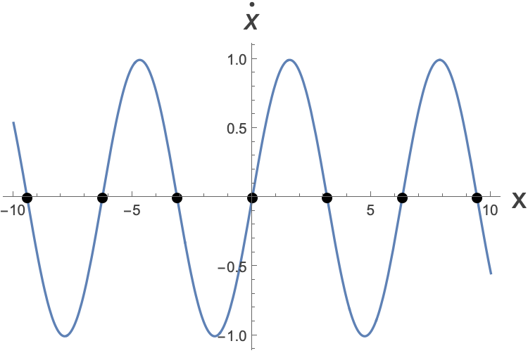
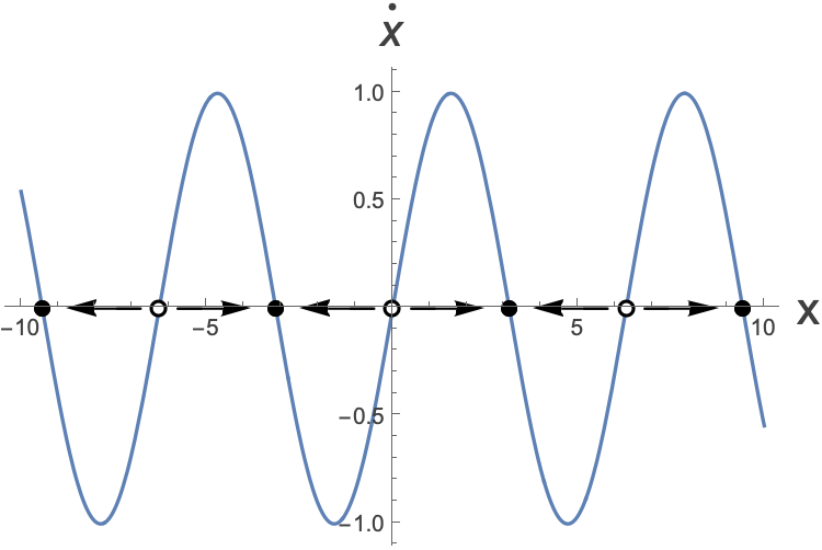
The first thing that we’re going to do is to plot $\dot{x} $against $x$. Well, in this case $\dot{x}$ is just $\text{ sin }\left(x\right)$, so we have:
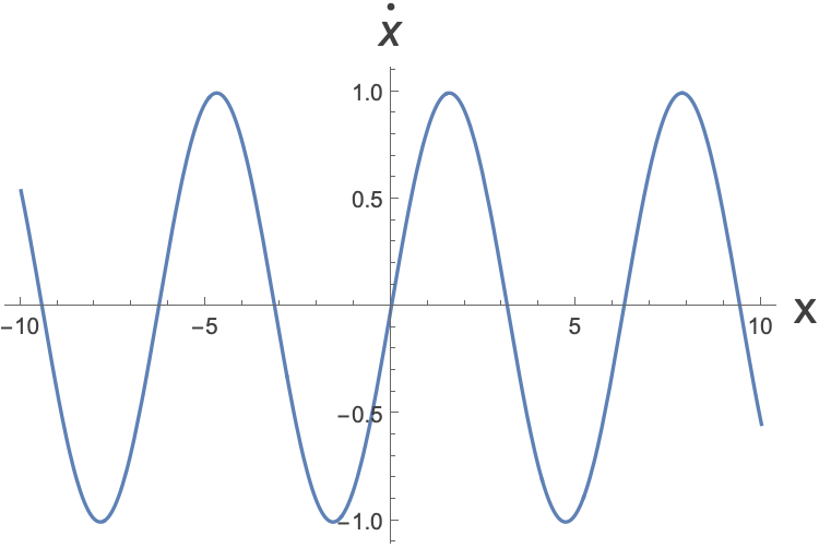
Well what does this mean?
- $\dot{x}$ tells us how fast we are moving along the line, for a given $x$ (the velocity). If we want to ask how fast we are going at, say the position $x=2$, we just read off the value of $\dot{x}$:
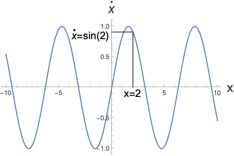
So the velocity of our particle, when we are at position $x=2$ is $\dot{x}=\text{ sin }\left(2\right)\approx{}0.91$ (i.e. moving right, with speed roughly 0.91). Now let’s ask the same question at $x=4$:
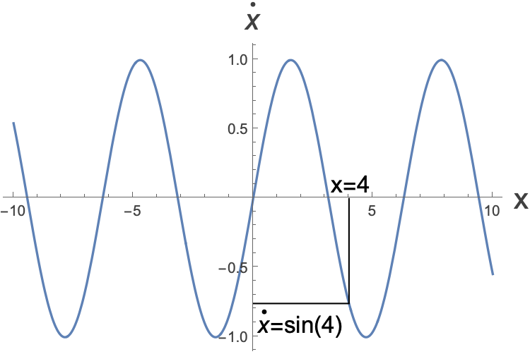
So the velocity of our particle, when we are at position $x=4$ is $\dot{x}=\text{ sin }\left(4\right)\approx{}-0.76$ (i.e. moving left, now at a slightly slower speed of 0.76)
In fact, we can see that whenever $\dot{x}$ is positive, we are moving to the right, and whenever $\dot{x}$ is negative we would be moving to the left. We put arrows on our line to show direction of motion in each region:
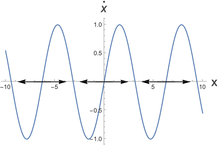
We can see something else from the plots. The closer we get to an intersection point of the sinusoidal curve with the x-axis, the smaller the magnitude of our velocity will be.
In fact, we can see that when we are at an intersection point, our velocity will be zero (i.e. $\dot{x}=0$). These are called Fixed Points. If a particle (a flow) starts at one of these special points, it never moves from it, hence it is fixed to the point.
For now, let’s put a black dot at every fixed point. In a bit we will see that not all fixed points are equal…
If I put you at a particular point. You could work out how fast and in which direction you would be moving, you can imagine going in that direction and then the next moment you will be somewhere else, and moving at a slightly different speed. Let ’s zoom into one region (between $x =0$ and $x=\pi{}$) and see what happens if I dropped you at just a little after $x=0$, let’s say at $x=0.1$. Our velocity at this point is going to be $\dot{x}=\text{ sin }\left(0.1\right)\approx{}0.1$ to the right.
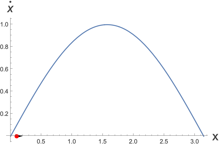
One really important thing to keep in mind, is that we are only moving along the x-axis. The vertical axis gives us information about how we are moving, but nothing more.
You can barely see the arrow (Size gives the magnitude). We will however, slowly move to the right. After a while you will get to $x=0.5$, at which point your velocity will have increased a bit.
When we get to $x=\frac{\pi{}}{2}$, we are speeding along to the right at our maximum velocity.
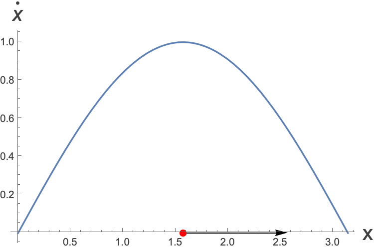
As we whizz past $x=\frac{\pi{}}{2}$, we start to slow down. so by the time we get to $x =3$, say, we are barely moving at all.
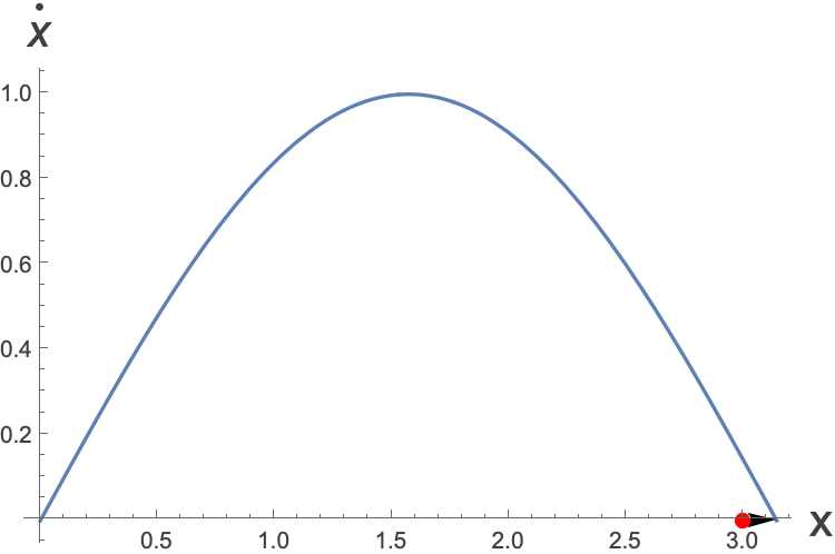
We edge ever close to $x=\pi{}$ but the closer we get, the slower we get and we… never… quite… make… it there… our destiny is to be forever moving to the right, slower and slower, without ever quite reaching $x=\pi{}$.
This same thing happens when starting at any point we want. There are certain points that you will always move away from, and certain points that you will always move towards (but never arrive at). The points that we move away from are called unstable fixed points, and those that you move towards are called stable fixed points.
Stability: The idea that small shakes or perturbations don’t cause large changes. If we start a particle/flow exactly on a fixed point, it never moves.
If we perturb the flow and it moves away from a fixed point then it is an unstable fixed point and if it moves back towards it then it is a stable fixed point.
Think of balancing a ball at the top of a hill.
- In theory you can balance perfectly there, but any little wobble and you will fall down (unstable)
Conversely, imagine a ball at the bottom of a valley.
- Any little push away and it will roll back down to the bottom of the valley (stable)
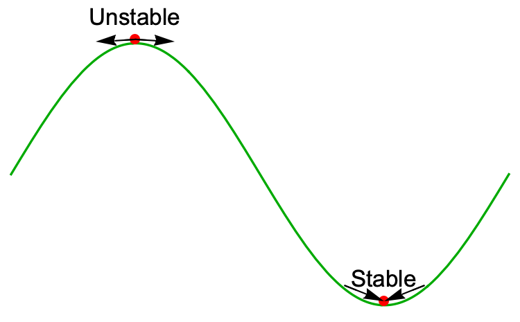
Note that a system like a ball on a hill is not the same as our one-dimensional system. However, to get an idea of stable and unstable fixed points it ’s a useful analogue.
We can label the stable and unstable fixed points separately:
A solid black disk at a stable fixed point.
An open circle at the unstable fixed point.
What are the trajectories going to look like starting with a particular initial condition?
To plot these, we don’t want $\dot{x}$ as a function of $x$. Instead we just want $x$ as a function of $t$. Let’s take the one that we went through in detail above, starting at $x=0.1$, and let’s say we start it at $t=0$. It’s going to look something like this:
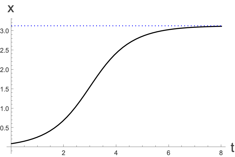
Make sure that you understand this. The asymptotic behaviour of $x\to \pi{}$ is given as the dashed line. Note that you can sketch this without having to know that complicated function that we wrote down above. We can see here is that the steepest point on the curve (i.e. when the velocity, or in other words $\dot{x}$ is highest) is when $x=\frac{\pi{}}{2}$. If you’re not sure, compare the phase portrait $\dot{x}$ values and the graph above’s gradient with it ’s $x$ values.
We can plot different trajectories on the same graph:
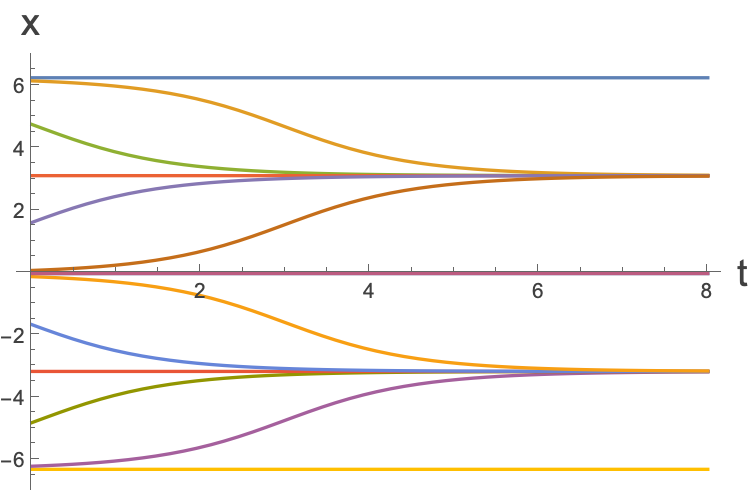
Spot the stable and unstable fixed points here!
And we can follow along with one of the trajectories to see what the actual particle motion looks like:
Click here to see the animation.
It looks like the particle makes it to the point $x=\pi{}$, but in reality as we said before, it never quite makes it.
Now let’s move on to a more general investigation of these methods.