1.4 Phase Space

Section 1.4: Phase Space

Phase Space

Let’s go back to the example of the pendulum. We said that the equation is governed by:

$$ x''\left(t\right)+\frac{g}{l}\text{ sin }\left(x\left(t\right)\right)=0 $$

In this course, x or y implies x(t) or y(t) respectively and they’re used interchangeably as the value of x is time dependent.

Before we called it θ not $x$ but that’s ok - it’s just changing the names of variables. Just for reference, you can solve this and it’s given by:

Where $c_{1}$and $c_{2}$ are constants of integration. This is something called a “Special Function” and you don’t need to know about it at all, but this is just to show that there is a solution even if it’s kinda complicated.

OK, so we’re going to use this example to understand about an idea called Phase Space. Let’s first of all take this second order equation and convert it to two first order equations.

• Let’s let $x_{1}\left(t\right)=x \left(t\right)$ and $x_{2}\left(t\right)=x' \left(t\right)$.

• We’re just relabeling $x_{ } $as $x_{1}$and we’re defining a new variable $x_{2}$ as the rate of change of $x/x_{1}$.

• Doing this gives us two equations:

$$ x_{1}'\left(t\right)=x_{2}\left(t\right) $$$$ x_{2}'\left(t\right)=-\frac{g}{l}\text{ sin }\left(x_{1}\left(t\right)\right) $$

Here we have two first order differential equations, and to solve them we will need two initial conditions, for $x_{1}\left(0\right)$ and $x_{2}\left(0\right)$.

• This would correspond to the initial angular position and angular velocity of the pendulum.

Now comes the fun part. We can now plot this position in a two dimensional plane, called the phase space of the problem. Let’s say that the initial angular position is $-\frac{\pi{}}{4}$and the initial angular velocity is -1. This would correspond to one position in the phase space and correspond to the pendulum at a certain point, swinging with a certain velocity.

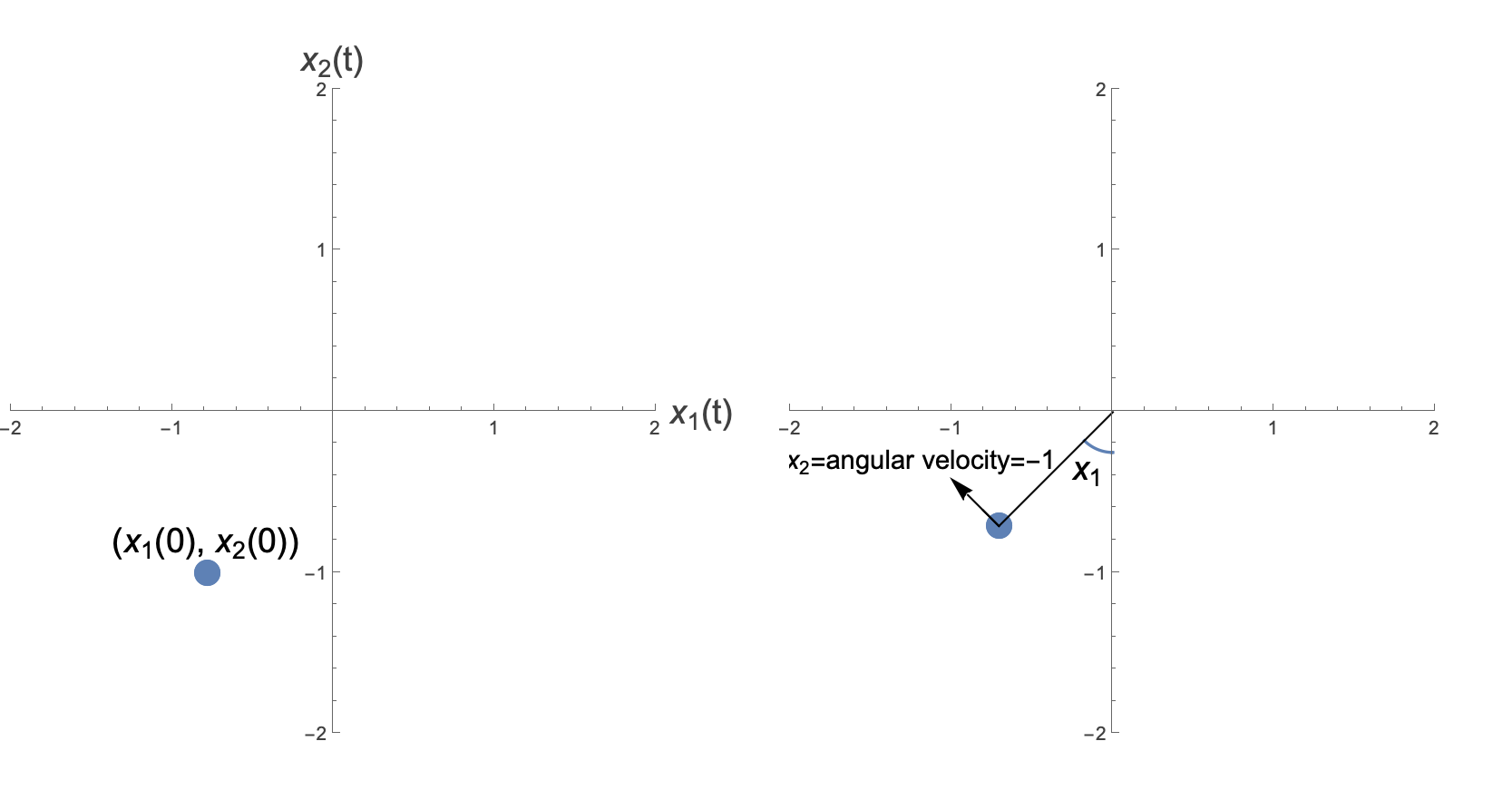
Remember, and this is key, that $x_{2}\left(t\right)$ is the angular velocity, and $x_{1}\left(t\right) \text{ is the }$ angle, they’re not positional co-ordinates.

So that is a single moment in time. As we roll time forward - ie. starting at that position in phase space/that initial angular position and velocity. It’s going to trace out a path in the phase space, which might look something like this:

Click here to see it visually!

On the left we see the path taken through phase space. At any one time the pendulum position is given by a single point in the phase space corresponding to a single position, and angular velocity. As we roll time forward, we move to different points in phase space. There are a few things to note:

1. The path in phase space is periodic - after a certain amount of time, we get back to where we started, not just in terms of position, but also velocity - That should make sense for a swinging pendulum.

2. When we cross the $x_{1} $axis, this corresponds to the moments where $x_{2}$is zero (angular velocity being zero). These points are when the pendulum has momentarily stopped at the far left and right of its swing.

This was a very particular starting position in phase space. Let ’s look at another:

Click here to see it visually!

This time we are starting with a slightly higher angular velocity (of -1.4, rather than -1) which is enough to take us slightly over the horizontal.

The point is that you can start anywhere in phase space that you want, and it will also give you some solution. Actually, let’s look at a whole range of solution all together in phase space:

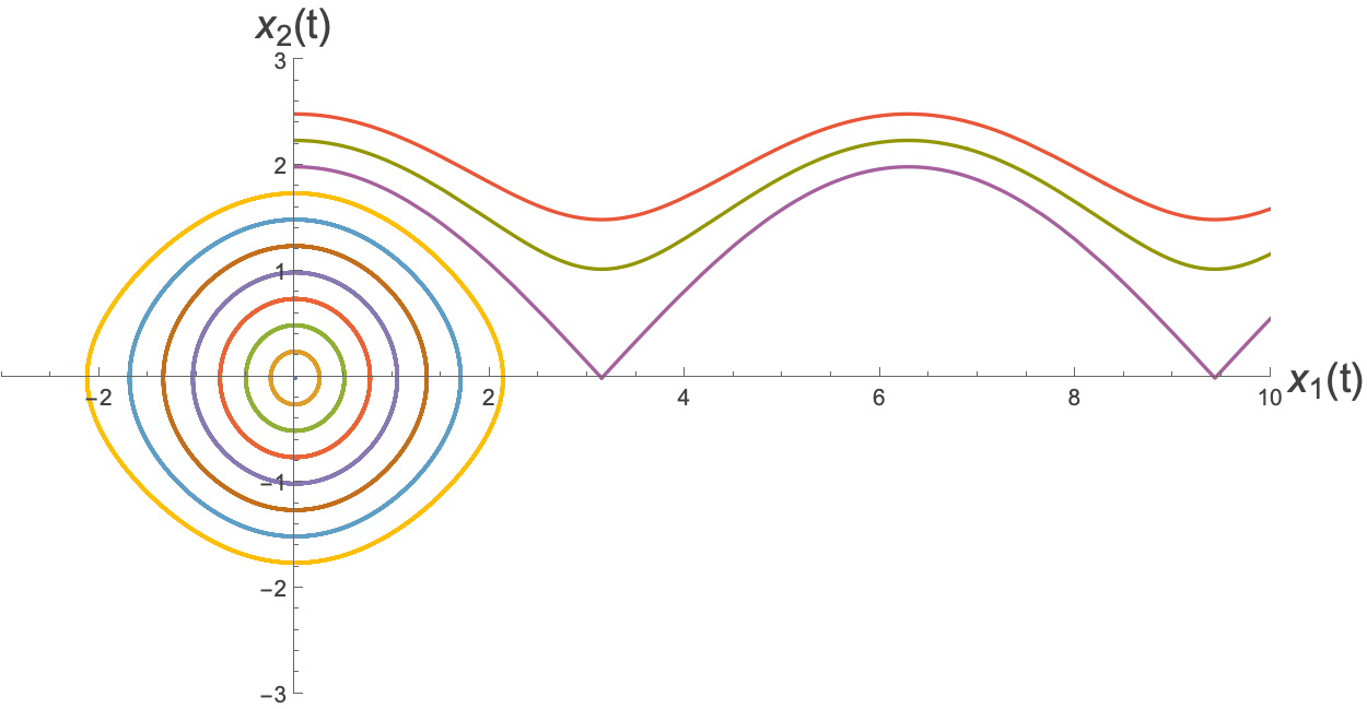
What is happening for higher and higher values of $x_{2}$ at $x_{1}$= 0?

So, phase space is a way to encode all of the possible states of the system. Every state of the system corresponds to a single point in phase space, and vice versa. Here we started with a second order differential equation and converted it to two first order equations, in $x_{1}$and $x_{2}$. This is why our phase space was two dimensional. One could end up with a higher dimensional phase space, and of course that is harder to plot.

In general if I give you a point in phase space you will be able to work out the future trajectory of the system.

We have to be careful about the difference between Position Space (a path in Position Space tells you where they are over time) and Phase Space which gives you the state of the particles, in terms of both their position and velocity. Phase Space plots out the full configuration of your system. It is more than just a snapshot of where things are, but also contains information at any one moment about how fast the particles are going. How fast they are going is how position is changing with time (linear velocity, angular velocity etc.). As the system moves through time, it traces out a path in Phase Space.

If we had a particle moving around in three dimensional space, then at any point in time, it can be completely described by its position and its velocity. Each of these is a three dimensional quantity, and so the phase space is six dimensional… and we’re not going to try and plot that.

If we had a box with gas in it, then there might be ${10}^{23 }$or so molecules in it. Each one of these will have a (3d) velocity vector as well as (3d) position vector associated with it, and moreover it may even be rotating ((3d) rotation vector as well as (3d) rotation velocity vector). So the whole system could be a $\left(3+3+3 + 3\right) {10}^{23} $phase space. Thankfully, it turns out that there are much better ways to describe gasses than this, and that is the study of statistical mechanics… and we’re not going there.

In fact in this course we are almost exclusively going to be dealing with one dimensional problems (which have a two dimensional phase space).

These types of problems are called “Problems on the Line” - because the position of our “Thing” is given by just a single number (like we had the angle of the pendulum above). The phase space is going to be 2d, and we’re going to see what we can discover about these systems without going to the hassle of solving the differential equations.

One little additional possibility that we haven’t considered is a system where the time is explicit in the equation itself. For instance:

$$ m x''\left(t\right)+b x'\left(t\right)+k x\left(t\right)=F \text{ cos } t $$

You can see that we have an explicit $t$-dependence on the right hand side. This says that there is something about the forces acting on our system that themselves are changing in time. In fact, this equation is more intuitively understood by rearranging it:

$$ m x''\left(t\right)=F \text{ cos } t-b x'\left(t\right)-k x \left(t\right) $$

Which says that the acceleration of the particle has three contributions - one related to how far it is from equilibrium (the last term) - the further from $x=0$ the more it accelerates towards that point. One related to how fast it’s going - the faster it’s going the more it will want to slow down quickly, and one which has a constant F (which you can think of as a force) multiplying something that varies in time. This is an external force on the system which accelerates it back and forth over time.

INTEREST QUESTIONS

What does an constant external force mean, physically?

Imagine a pendulum. A frictional force will slow it down over time, and eventually, stop it.

• Now imagine yourself pushing on the pendulum in a periodic motion with your finger. This would be an external periodic force on the system.

• There may be some balance whereby the external forcing motion counters the effects of the friction so that it never stops.

• If there was no friction in this example then your forcing motion on the system may just keep accelerating it for ever…

Can we write this in the form of a system of 1d equations without the t being present explicitly?

We are going to be very sneaky, and as well as doing what we did before by defining $x_{1}\left(t\right)=x\left(t\right)$ and $x_{2}\left(t\right)=x'\left(t\right)$, we are going to define a new variable $x_{3}\left(t\right)=t$. So of course $x_{3}'\left(t\right)=1$.

Now we can write down our system as:

$$ x_{1}'\left(t\right)=x_{2}\left(t\right) $$$$ x_{2}'\left(t\right)=\frac{1}{m}\left(-k x_{1}\left(t\right)-b x_{2}\left(t\right)+F \text{ cos } x_{3}\left(t\right)\right) $$$$ x_{3}'\left(t\right)=1 $$

A system which has explicit time-dependence is called a non-autonomous system (or simply time-dependent). In general we can take an $n^{\text{ th }}$order non-autonomous differential equation and convert it into a system of (n+1) first order, autonomous (not explicitly depending on time) differential equations, as we have done above.

There’s something rather interesting about a forced system like this. Let’s see what happens when we change the initial conditions. Here we take an example where F = 0.5, k = 0.5 and b = 1.5 and solve it with different values of $x \left(0\right)$ and $x'\left(0\right)$.

Note importantly, you are NOT expected to be able to solve these equations within this course. This is an example to show you what a forcing term does for you.

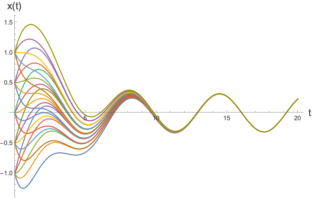
You can see that there is some initial behaviour which is dependent on the initial conditions (this is called transient behaviour) and following this it settles down to a steady-state behaviour which is determined by the forcing term.

Would you ever have acceleration/need it as a direction in phase space?

In the examples we’ve given, phase space informs the position and the velocity of our system. The equation of motion (the original differential equation) generally gives you a link between acceleration, velocity and position, so if you know position and velocity in the phase space, the acceleration is already determined for you.

For most of what we will be covering in this course, the phase space will be even simpler. If we are looking at a single first order equation, then the velocity is determined by the position, so phase space is one dimensional.

We would need a direction in phase space for acceleration if you had a third order differential equation, say:

$$ p x'''\left(t\right)+m x''\left(t\right)+b x'\left(t\right)+k x \left(t\right)=0 $$

Here there is a third derivative, so if given just the position and velocity, the acceleration is NOT determined. Here you would need the position, the velocity, and the acceleration to determine the evolution of the system, so in this case the phase space would be three dimensional.

What are these ‘degrees of freedom ’ which keep getting mentioned?

The degrees of freedom of a system are the variables which define the state of the system which can vary independently. So, for instance for the pendulum, the position and angular velocity are “degrees of freedom” because you can set them independently and it’s a perfectly well defined state of the system. The acceleration is however not a degree of freedom, because once you’ve chosen the position and velocity, you are not free to choose the acceleration. It’s dictated by the equation of motion.

The number of degrees of freedom is the dimension of the phase space. This is also equal to the number of first order autonomous differential equations which describe the system.