What we'll cover
The reinforcement-learning vocabulary used here (policy, episode, reward, advantage) is set out in the primer in 6.1. We have a policy (the SFT model) and a reward model \(r_\phi\). Step 3 of RLHF optimises the policy to score highly under \(r_\phi\). This sub-session writes down the actual objective (reward minus a KL penalty), explains why that penalty (the "leash") is doing the real safety work, sketches PPO, the RL algorithm that performs the optimisation, and introduces DPO, which reaches a similar place without explicit RL. The recurring theme: how hard you optimise a proxy is itself a safety dial.
Mandatory readings
• DeepSeek-AI (2025), "DeepSeek-R1: Incentivizing Reasoning Capability in LLMs via Reinforcement Learning" (arXiv:2501.12948): §2.2.1, the GRPO objective, and §2.2.2, the rule-based rewards it optimises. Read it after the GRPO section below, where the equation should be legible: it is PPO's clipped ratio with the group mean standing in for a critic. ≈700 words.
• Schulman et al. (2017), "Proximal Policy Optimization Algorithms" (PPO; arXiv:1707.06347): read §3 (Clipped Surrogate Objective) for the one idea you need from PPO: keep each policy update small by clipping the probability ratio. Read it for the shape of the argument, not the algebra. Nothing later in the course asks you to reproduce the clipped objective, and the figure further down this page marks what you can pass over. ≈550 words.
• Rafailov et al. (2023), "Direct Preference Optimization" (NeurIPS 2023; arXiv:2305.18290): read §4 (Direct Preference Optimization), the derivation that removes the separate reward model. ≈1,050 words.
Total mandatory load: ≈2,300 words.
Optional readings
• Yue et al. (2025), "Does Reinforcement Learning Really Incentivize Reasoning Capacity in LLMs Beyond the Base Model?" (arXiv:2504.13837): the pass@k evidence that current RLVR may elicit base-model capability rather than extend it.
• Bai et al. (2022) (arXiv:2204.05862): the reward-versus-\(\sqrt{\mathrm{KL}}\) relationship and how the KL penalty behaves in practice.
• Rafailov et al. (2023) (arXiv:2305.18290), §5: the theoretical analysis, including why a language model is secretly a reward model.
The RLHF objective
Naïvely, we'd just maximise expected reward. That is the way to get burned by the proxy, so we add a brake.
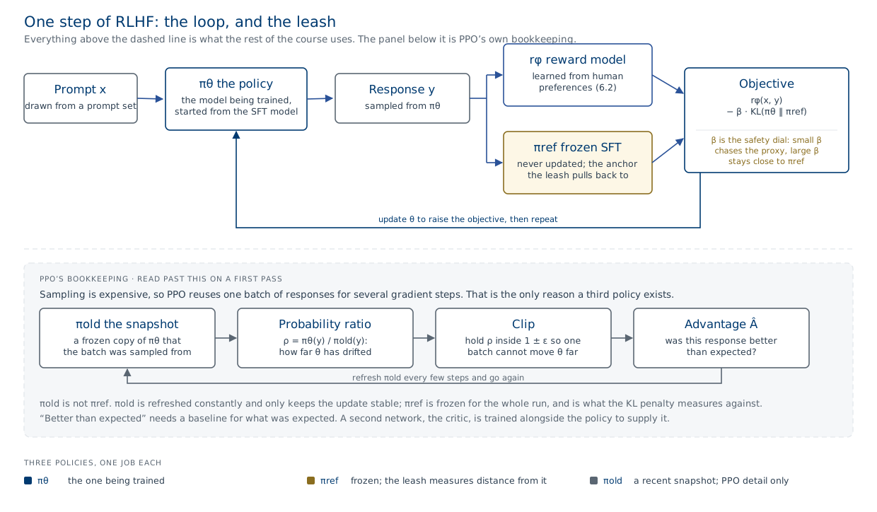
Let \(\pi_\theta\) be the policy we are training and \(\pi_{\text{ref}}\) the frozen SFT model we started from. The standard RLHF objective maximises expected reward on prompts \(x\) and sampled responses \(y\sim\pi_\theta\), penalised by how far the policy has drifted from \(\pi_{\text{ref}}\), measured by Kullback–Leibler divergence:
Kullback–Leibler divergence measures how far one distribution has moved from another: \(\mathrm{KL}(\pi_\theta\|\pi_{\text{ref}}) = \mathbb{E}_{y\sim\pi_\theta}\big[\log \pi_\theta(y\mid x) - \log \pi_{\text{ref}}(y\mid x)\big]\), the average log-ratio the policy assigns to its own samples against what the reference model would have assigned. It is zero when the two agree everywhere and grows as they separate. It is not symmetric, and this direction punishes the policy for putting weight where the reference model puts almost none. Its unit is the nat, which is what the 6.5 lab reports. The coefficient \(\beta\) sets the strength of the leash. With \(\beta=0\) the policy is free to chase reward anywhere; large \(\beta\) keeps it almost identical to the SFT model. RLHF lives in between.
The KL penalty
The two jobs of the KL term
The reward model is a proxy, accurate only near the responses it was trained on (6.2). An unconstrained optimiser will happily march into regions where the proxy is high but wrong: degenerate, repetitive, or manipulative text that the reward model mistakenly loves. The KL term forbids that: it keeps the policy in the neighbourhood of the SFT model, where the reward model's judgements are trustworthy and the outputs stay fluent. So the KL penalty is doing two safety jobs at once: preserving the language competence inherited from pretraining/SFT, and limiting how far we trust an imperfect reward. It is a direct, tunable handle on "how hard do we dare optimise the proxy?".
An empirical regularity
Bai et al. (2022) report that, across RLHF runs, the reward achieved grows roughly linearly with \(\sqrt{\mathrm{KL}}\): the further the policy moves from its initialisation (in root-KL), the more reward it gains, predictably. That is useful two ways: it gives a principled axis for "how much optimisation" you've applied, and (paired with the over-optimisation result in 6.4) it lets you see true quality peak and then fall along that same \(\sqrt{\mathrm{KL}}\) axis. The leash and the curse are measured in the same units.
Worked example: what β buys
Use that regularity. Model the reward gained as \(R(d) = d\), where \(d = \sqrt{\mathrm{KL}}\) measures how far the policy has moved from \(\pi_{\text{ref}}\); the square root is the convention throughout this literature, and 6.4 and the lab use the same \(d\). The KL penalty costs \(\beta\,\mathrm{KL} = \beta d^{2}\), so the penalised objective is \(d - \beta d^{2}\); setting its derivative to zero gives \(1 = 2\beta d\), so the optimiser settles at \(d^{*} = \tfrac{1}{2\beta}\), reaching reward \(\tfrac{1}{2\beta}\). Read the consequence straight off: \(\beta = 0.5\) sends the policy to \(d^{*}=1\), while dropping \(\beta\) to \(0.25\) lets it run out to \(d^{*}=2\), four times the KL distance: halving the leash quadruples the distance travelled and doubles the reward collected. So \(\beta\) is not a vague stability knob; it sets, quantitatively, how hard you optimise the proxy. The twist 6.4 adds is the one this toy omits: the true reward does not climb like \(\sqrt{d}\) forever; it peaks and turns down, so pushing \(d^{*}\) higher eventually makes the model worse even as the proxy reward keeps rising.
RLHF with β = 0
Set \(\beta = 0\) and let the optimiser run, and RLHF reliably produces degenerate text: outputs the reward model scores very highly but a human finds absurd, such as a fixed phrase the reward model happened to love, repeated; strange formatting; or fawning, content-free agreement. The policy has found a corner of output-space where the proxy is wrong and exploited it: Session 3.1's specification gaming, live. The KL penalty prevents this not by improving the reward model but by forbidding the policy from travelling to the regions where the reward model's errors live, keeping it near fluent, SFT-like text where the proxy can still be trusted. That is why "how hard you optimise" is a safety dial, not just a performance one.
PPO, briefly
The objective says what to maximise; PPO is how. You do not need its full derivation, but you should know what it is and why it's used.
Proximal Policy Optimization (Schulman et al., 2017)
RLHF is a reinforcement-learning problem: the policy generates a response (a sequence of actions = tokens), receives a reward, and we want to nudge it toward higher-reward responses. The difficulty is that large policy-gradient steps are unstable: push too hard on one batch and the policy can collapse. PPO solves this with a clipped surrogate objective: it allows the policy to change only within a trust region of the previous policy each update (clipping the probability ratio so updates that move too far are not rewarded). This buys the stability of more complex methods (like TRPO) with simple first-order optimisation, and it is the workhorse RL algorithm in the InstructGPT pipeline. PPO is a careful, small-step climber of the KL-penalised reward, itself a second mechanism for "don't move too fast".
Concretely, PPO looks at the probability ratio \(\rho = \pi_\theta(a)/\pi_{\text{old}}(a)\) between the new policy and \(\pi_{\text{old}}\), the snapshot in the panel of the figure above (not the frozen \(\pi_{\text{ref}}\) the leash measures against), for each token, weighted by an estimated advantage \(\hat{A}\) (how much better that token turned out than expected), and optimises \(\min\!\big(\rho\hat{A},\ \operatorname{clip}(\rho,\, 1-\epsilon,\, 1+\epsilon)\,\hat{A}\big)\). With \(\epsilon = 0.2\), a token whose advantage is positive but whose ratio has jumped to \(\rho = 1.5\) is treated as if \(\rho = 1.2\): moving further earns no extra objective, so the step is reined in. The clip is a per-update trust region; the KL penalty is the global leash. Two brakes, at two scales.
GRPO: dropping the critic
Group Relative Policy Optimization (Shao et al., 2024)
PPO needs a critic to say what score was expected, and that critic is a second network, typically the same size as the policy. You are training two large models to improve one. GRPO removes it. Instead of learning to predict the expectation, it samples several answers to the same question and lets the group tell you what was expected.
For a question \(q\), sample a group of \(G\) responses from the current policy and score them all. The advantage of response \(i\) is then measured against its own group:
A response that beat the others in its group gets a positive advantage and is made more likely; one that lagged them is made less likely. Everything else carries over from PPO unchanged: the same clipped probability ratio keeps each step small, and the same \(\beta\,\mathrm{KL}(\pi_\theta \,\|\, \pi_{\text{ref}})\) leash holds the policy near the reference model. Only the baseline changed, from a learned prediction to the mean of a handful of siblings.
It is the algorithm behind the reasoning models of 5.3's stage 4. When the reward is a checker rather than a person, sampling twenty attempts at the same maths problem costs almost nothing, so a group is cheap to come by, and what PPO spends an extra network estimating can be read straight off the sample. Sampling many answers per question also suits a task where most attempts fail and only the occasional one succeeds.
You have already seen an implementation. scripts/chat_rl.py, the file you searched in the 5.4 lab, runs GRPO on grade-school maths, and its docstring is candid about how much it strips out: no KL term, no ratio and clip (it stays on-policy, so the ratio is 1), and the plain difference \(r_i - \operatorname{mean}(r)\) in place of the division by the standard deviation. What survives all that is the group baseline.
Practice has already moved past GRPO itself. DAPO (arXiv:2503.14476) and GSPO (arXiv:2507.18071) both change the details, GSPO by clipping on whole sequences rather than tokens, which it reports as stabilising training for the mixture-of-experts models of 2.2. Frontier labs do not disclose what they run. What has survived every version is the idea in the paragraph above: drop the critic, and take the baseline from a group of samples. That is why R1 is still the right paper to learn it from.
Reading the objective
Here is the whole thing, as §2.2.1 of the paper writes it. Nothing in it is new. It is the pieces above, assembled.
Work from the outside in.
- The expectation. The bracket after \(\mathbb{E}\) is a list of what you are averaging over, not a product of two quantities. Read it as an instruction: draw a question \(q\) from your pool of training questions \(P(Q)\), then draw a group of \(G\) answers \(\{o_1,\dots,o_G\}\) to that one question from \(\pi_{\theta_{\text{old}}}\). One question, \(G\) answers, and the objective is the average over many such draws. \(G\) is a small number in practice, 8 or 64.
- The group average. \(\frac{1}{G}\sum_i\) says each of those \(G\) answers contributes one term, weighted equally. This is the sum whose mean also defines \(A_i\), which is why the group has to be sampled before anything else can be computed.
- The ratio \(\rho_i = \pi_\theta(o_i \mid q) \,/\, \pi_{\theta_{\text{old}}}(o_i \mid q)\). The probability the policy being trained assigns to answer \(o_i\), over the probability the sampling policy assigned to the same text. At the first gradient step on a batch the two are the same network, so \(\rho_i = 1\) exactly. It drifts away from 1 as you take further steps on that same batch, and that drift is the only reason \(\pi_{\theta_{\text{old}}}\) appears at all.
- The advantage \(A_i\). The group-relative score from above: how far this answer beat its siblings, in standard deviations.
That leaves the two terms inside the sum.
The min and the clip
The usual gloss, that clipping holds the ratio inside \(1 \pm \varepsilon\), is not quite what the expression does. Take \(\varepsilon = 0.2\) and tabulate the bracketed term for a good answer and a bad one:
| \(\rho_i\) | \(A_i = +1\) (good answer) | \(A_i = -1\) (bad answer) |
|---|---|---|
| 0.5 | 0.50 | −0.80 |
| 0.8 | 0.80 | −0.80 |
| 1.0 | 1.00 | −1.00 |
| 1.2 | 1.20 | −1.20 |
| 1.5 | 1.20 | −1.50 |
| 2.0 | 1.20 | −2.00 |
For a good answer the objective stops rising once \(\rho_i\) passes \(1.2\), so there is nothing to gain by pushing its probability higher. For a bad answer it stops falling once \(\rho_i\) drops below \(0.8\), so there is no extra credit for crushing it further. But look at the bottom right: if an update raises the probability of a bad answer, the penalty keeps growing without limit.
That asymmetry is deliberate. The \(\min\) always takes the pessimistic branch, which makes the whole expression a lower bound on the improvement you are trying to make. Moving in the direction you want buys nothing beyond the band; moving in the direction you do not want is punished in full. "Trust region" names that, rather than a symmetric clamp.
Then \(-\beta\,\mathbb{D}_{\mathrm{KL}}(\pi_\theta \| \pi_{\text{ref}})\) is the leash from earlier on this page. Note that the objective now carries two different reference points doing two different jobs: \(\rho_i\) compares against \(\pi_{\theta_{\text{old}}}\), a snapshot from minutes ago, to keep the optimiser stable; the KL compares against \(\pi_{\text{ref}}\), frozen since the start of training, to keep the model close to the one that was aligned.
Why the KL term does not look like a KL
The paper does not write the KL as an expected log-ratio. It writes, with \(r = \pi_{\text{ref}}(o_i \mid q) / \pi_\theta(o_i \mid q)\),
which is not a typo and not a different divergence. It is an estimator of the same KL, due to Schulman, and it has two properties the obvious estimator lacks. Averaged over samples from \(\pi_\theta\) it is unbiased, and it is never negative, whereas \(-\log r\) is unbiased but goes negative on individual samples, which is awkward for a quantity you are reporting as a distance. It is also far quieter: on a small worked example with a true KL of \(0.0253\), both estimators recover it, but the variance of \(r - \log r - 1\) is about two hundred times smaller.
Do it once by hand: expand \(r - \log r - 1\) around \(r = 1\) and you get \(\tfrac{1}{2}(r-1)^2\) to leading order, which is why it is small and positive whenever the two policies nearly agree.
The pass@k debate
How much does this stage add? Yue et al. (2025) compare RLVR-trained models against the base models they were built from, at large sampling budgets, and find the base model often matches or overtakes the RL-trained one on pass@\(k\) (the chance that at least one of \(k\) independent samples is correct) as \(k\) grows. Read that way, current RLVR mostly improves which solutions get selected from the range a base model could already reach, rather than extending that range.
The debate is open, and it bears on 5.3's claim that the alignment layer is thin: if RL on verifiable rewards elicits rather than extends, then much of what a reasoning model does was already in the base model, waiting to be sampled well. This also raises the question of what an open-weight release actually releases.
DPO: preference optimisation without RL
Direct Preference Optimization (Rafailov et al., 2023)
RLHF's three-stage machinery (train a reward model, then run PPO with sampling) is fiddly and unstable. DPO observes that, for the KL-penalised objective above, the optimal policy has a closed form in terms of the reward and \(\pi_{\text{ref}}\), so one can rearrange and optimise the policy directly on the preference pairs, with a simple classification-style loss, no separately trained reward model and no RL sampling loop. "Your language model is secretly a reward model": the policy implicitly encodes the reward. The closed form is \(\pi^{*}(y\mid x) \propto \pi_{\text{ref}}(y\mid x)\,\exp\!\big(r_\phi(x,y)/\beta\big)\); DPO rearranges it to express the reward in terms of \(\pi_\theta\) and \(\pi_{\text{ref}}\), then substitutes that into the Bradley–Terry loss of 6.2, so the preference pairs train the policy directly. DPO matches or beats PPO-based RLHF on many tasks while being markedly simpler and more stable, and is now widely used. Conceptually, though, it is optimising the same preference-derived objective, so the proxy hazards of 6.4 still apply; DPO changes the how, not the what.
From the closed form to a loss
The \(\propto\) above is hiding the step that makes DPO work. Written out, the optimal policy is
That normalising constant \(Z(x)\) is a sum over every response the model could produce. There is no computing it, and if the method needed it there would be no method.
Rearrange for the reward instead of the policy:
Now recall from 6.2 that the Bradley–Terry model never sees a reward on its own. It sees only the difference between two of them, \(r(x,y_w) - r(x,y_l)\). And \(Z(x)\) depends on the prompt alone, not on which response is being scored, so it takes the same value in both terms and subtracts away. The intractable quantity is never needed.
What remains, writing \(\pi_\theta\) for the policy being trained, is an ordinary logistic loss on two log-ratios:
Set it beside the reward-model loss of 6.2 and the shape is the same. Only the contents of \(\sigma\) changed: where 6.2 had two reward-model scores, this has the policy’s own log-probability ratio against the frozen reference. That is what “your language model is secretly a reward model” means, written as an equation. No reward model is trained, nothing is sampled during training, and \(\beta\) still sets how far the policy may drift from \(\pi_{\text{ref}}\), exactly as it did in the RLHF objective at the top of this page.
DPO and the preference signal
It is tempting to read DPO as "RLHF without the danger". It isn't. DPO still fits the model to human preference comparisons and still pushes it toward what raters preferred; sycophancy and over-optimisation (6.4) arise from the preference signal, not specifically from PPO. Simplifying the optimiser doesn't remove the gap between "what raters prefer" and "what is good".
Questions to bring to class
- Explain, in terms of the reward model being a proxy, why setting \(\beta=0\) (no KL penalty) would be dangerous even with a "good" reward model.
- The KL penalty does two jobs. Name them, and say which is about capability and which is about safety.
- Bai et al. find reward \(\propto \sqrt{\mathrm{KL}}\). Why is having a single measured axis ("how far we've optimised") useful for studying over-optimisation (6.4)?
- DPO removes the explicit reward model and RL loop. Which RLHF risks does that remove, which does it leave untouched, and why?
Next
We can now train an assistant with RLHF. Sub-session 6.4 asks the safety question head-on: what goes wrong? Reward hacking, over-optimisation, sycophancy, and the difficulty of obtaining reliable feedback on tasks beyond unaided raters.