Session 2.1 — From neurons to networks

Week 1 — deep learning & scaling laws

To reason about how these systems fail, you need a working picture of how they're built. This session rebuilds that picture at the level a mathematician wants (functions, parameters, gradients), then shows why capability scales so predictably with size.

This session's sub-sessions: 2.1 from neurons to networks · 2.2 inside the transformer · 2.3 neural scaling laws · 2.4 pace of progress, emergence and takeoff · 2.5 lab (Colab).

What we'll cover

You have met neural networks before, but cohorts vary, so we set a common, precise baseline. This sub-session frames a network as a parametrised function fit by gradient descent (nothing mystical) and pins down the few ideas (the loss, the gradient, the objective) that the safety arguments later hang on.

Mandatory readings

• Watch: Karpathy, "The spelled-out intro to neural networks and backpropagation" (Zero to Hero, episode 1; embedded below): from the embedded timestamp (assembling neurons into a network) through the loss-function section. ~65 min video.

Total mandatory load: ~65 min of video.

Optional readings

• Refresher: 3Blue1Brown, "Neural Networks" video series: clear visual intuition for gradient descent and back-propagation.

• Refresher: any standard deep-learning text chapter on feed-forward networks and back-propagation (e.g. Goodfellow, Bengio & Courville, Deep Learning, Ch. 6).

Core material

The primary resource for this sub-session is Andrej Karpathy's spelled-out introduction to neural networks and backpropagation (Zero to Hero, episode 1), which builds the same ideas one neuron at a time, in code. Watch from the embedded timestamp (assembling neurons into a network), then the loss-function section. The page below is the written reference for the same material.

A complementary written treatment at the same neuron-by-neuron level: "Neurons", Structure of Deep Networks (Bau Lab).

A network is a parametrised function

Strip away the biology metaphor and a neural network is a function \( f_\theta : \mathbb{R}^n \to \mathbb{R}^m \) with a great many parameters \( \theta \).

From a neuron to a layer

Start with a single neuron: it takes an input vector \( x \in \mathbb{R}^{d_{\text{in}}} \), forms a weighted sum with its own weight vector \( w \) and bias \( b \), and passes the result through a nonlinearity, producing one scalar: \( a = \sigma(w \cdot x + b) \). Now stack \( d_{\text{out}} \) neurons side by side and collect their weight vectors as the rows of a matrix \( W \). The whole layer then computes a vector in one shot:

\[ h = \sigma(Wx + b), \qquad W \in \mathbb{R}^{d_{\text{out}} \times d_{\text{in}}}, \quad b,\, h \in \mathbb{R}^{d_{\text{out}}} \]

Here \( \sigma \) is applied elementwise (the same scalar function to each component), and the standard choice is ReLU, \( \sigma(z) = \max(0, z) \). A deep network chains \( L \) such layers, each feeding the next:

\[ h^{(\ell)} = \sigma\!\left(W^{(\ell)} h^{(\ell-1)} + b^{(\ell)}\right), \qquad h^{(0)} = x \]

and the full collection of weights and biases \( \{W^{(\ell)},\, b^{(\ell)}\} \) is what we bundled into the parameters \( \theta \). Without \( \sigma \) the composition of linear maps would collapse to a single linear map; the nonlinearity is what lets depth buy expressive power. By the universal-approximation results such a network can approximate essentially any function; the engineering question is whether gradient descent can find parameters that do so.

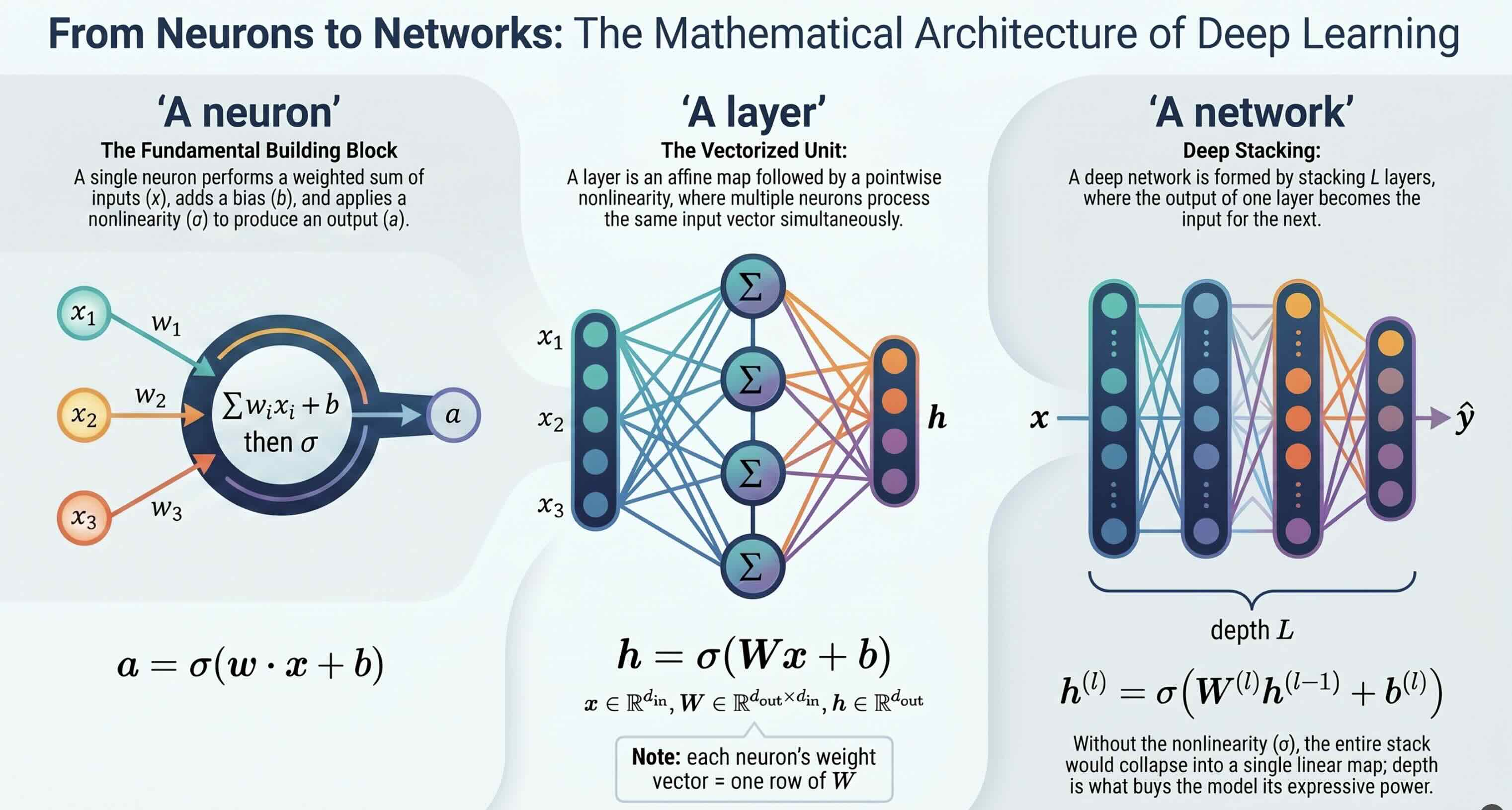
Three panels. (A) A single neuron: inputs x1, x2, x3 with weights w1, w2, w3 feed a node that computes the weighted sum plus a bias and then a nonlinearity, giving the scalar a = σ(w·x + b). (B) A layer: an input vector fully connected to a column of neurons, producing the vector h = σ(Wx + b), with x in ℝ^d_in, W in ℝ^(d_out×d_in) and h in ℝ^d_out, and each neuron's weight vector forming one row of W. (C) A network: several such layers stacked left to right, with x entering and ŷ leaving, computing h^(l) = σ(W^(l) h^(l−1) + b^(l)) over depth L. — **From a neuron to a network.** (A) one neuron, \( a = \sigma(w \cdot x + b) \); (B) a layer stacks neurons into \( h = \sigma(Wx + b) \), where each neuron's weights are one row of \( W \); (C) a deep network chains \( L \) such layers. Without the nonlinearity the whole stack would collapse to a single linear map.

A forward pass by hand

Make the layer concrete with one neuron. Take input \(x = (1,\, 2,\, -1)\) and a neuron with weights \(w = (0.5,\, -1,\, 2)\) and bias \(b = 0.5\). Its pre-activation is \(w\cdot x + b = (0.5)(1) + (-1)(2) + (2)(-1) + 0.5 = -3\), and with ReLU the output is \(\sigma(-3) = \max(0,-3) = 0\); this neuron is "off" for this input. A second neuron with \(w' = (1,1,1)\) and \(b'=0\) gives \(w'\cdot x = 2\), so \(\sigma(2)=2\). Stack the two and the layer outputs \((0,\,2)\). A whole network is just this, repeated: hundreds of billions of such weighted sums and ReLUs, arranged in layers. Nothing in a forward pass is more exotic than what you just did by hand.

Collapse without a nonlinearity

Here is why \(\sigma\) is not optional. Drop it, and two layers compose to \(W_2(W_1 x + b_1) + b_2 = (W_2 W_1)\,x + (W_2 b_1 + b_2)\), which is just one affine map \(W' x + b'\). Without a nonlinearity, a network of any depth collapses to a single linear layer and can only draw straight decision boundaries; no amount of stacking buys anything. Insert ReLU between the layers and the collapse is blocked: each layer bends the input space along a different set of hyperplanes, and composing many such bends lets the network carve the highly non-linear regions real data lives in. That is the formal content behind "depth buys expressive power", and the reason every block in a transformer (2.2) carries a nonlinearity.

Training = minimising a loss

"Learning" is optimisation. We choose a loss that scores predictions against targets and descend it.

The training loop

Loss. A scalar \( L(\theta) \) measuring how wrong the model is on data: for language models, the cross-entropy of the predicted next-token distribution against the true token.
Gradient. Compute \( \nabla_\theta L \) by back-propagation (the chain rule, applied layer by layer).
Step. Update \( \theta \leftarrow \theta - \eta\, \nabla_\theta L \) for a small learning rate \( \eta \) (in practice, a variant like Adam). Each step estimates the gradient on a mini-batch (a small random subset of the data, far cheaper than using all of it), and we repeat for a very long time.

That is all of it. Everything a frontier model "knows" is the low-loss configuration of \( \theta \) this process settles into on its training data.

Gradient descent and back-propagation

The gradient \( \nabla_\theta L \) points in the direction in parameter space along which the loss rises fastest, so stepping the other way lowers it, with the learning rate \( \eta \) setting the step size. Back-propagation is the chain rule organised so that one backward pass, costing about as much as one forward pass, yields the gradient for all the parameters at once. That is what makes training billion-parameter models feasible at all. Two caveats matter later. The loss surface is wildly non-convex, so this finds a low-loss region, not the global minimum, and which region depends on the initialisation and the order of the data. And the result is a vast array of numbers that happens to fit the data, with no guarantee of being readable: gradient descent optimises for low loss, never for interpretability. Both points come back in Session 3 and in the interpretability weeks.

The language-model loss

A language model is trained to predict the next token (a chunk of text, defined precisely in Session 2.2) given the tokens before it. At each position it outputs a probability distribution \( p_\theta \) over the whole vocabulary (the softmax of its output scores; softmax is defined in 2.2), and the loss is the cross-entropy:

\[ L = -\frac{1}{T} \sum_i \log p_\theta\!\left(t_i \mid t_{<i}\right) \]

where \( t_i \) is the true token at position \( i \) and \( t_{<i} \) all tokens before it. (General cross-entropy is \( -\sum p_{\text{true}} \log p_\theta \); because the true "distribution" puts all its mass on the one token that occurred, the sum collapses to the negative log-probability of that token.) So minimising \( L \) means making the correct token as probable as possible. Two things follow: this is the "loss" that falls as a power law in Session 2.3; and the model is never told how to be right, only scored on the probability it placed on what came next.

Consequences for safety

We specify the loss; the optimiser finds the behaviour

The rest of the course turns on this. We do not program behaviour; we specify a loss and an optimiser, and behaviour is whatever minimises that loss on that data. The model optimises the objective we wrote down, which is only ever a proxy for what we meant. Every alignment failure you'll study is, at root, a gap between those two, surfaced by an optimiser doing its job.

Specification and opacity

First, the objective is a specification problem: get the loss subtly wrong and you get subtly wrong behaviour, at scale (Session 3, Goodhart). Second, the parameters are opaque: gradient descent finds a solution, not an interpretable one, which is why we need mechanistic interpretability (Weeks 7–8) to read back out what the network learned.

The networks behind modern AI have a specific architecture: the transformer. Sub-session 2.2 opens it up, with the attention mechanism and the residual-stream view we'll reuse when we get to interpretability.